Journal of Software Engineering and Applications
Vol.7 No.7(2014), Article
ID:46575,9
pages
DOI:10.4236/jsea.2014.77052
NeuroEvolutionary Feature Selection Using NEAT
Soroosh Sohangir, Shahram Rahimi, Bidyut Gupta
Computer Science Department, Southern Illinois University Carbondale, Carbondale, USA
Email: ssohangir@cs.siu.edu, Rahimi@cs.siu.edu, bidyut@cs.siu.edu
Copyright © 2014 by authors and Scientific Research Publishing Inc.
This work is licensed under the Creative Commons Attribution International License (CC BY).
http://creativecommons.org/licenses/by/4.0/


Received 22 April 2014; revised 15 May 2014; accepted 23 May 2014
ABSTRACT
The larger the size of the data, structured or unstructured, the harder to understand and make use of it. One of the fundamentals to machine learning is feature selection. Feature selection, by reducing the number of irrelevant/redundant features, dramatically reduces the run time of a learning algorithm and leads to a more general concept. In this paper, realization of feature selection through a neural network based algorithm, with the aid of a topology optimizer genetic algorithm, is investigated. We have utilized NeuroEvolution of Augmenting Topologies (NEAT) to select a subset of features with the most relevant connection to the target concept. Discovery and improvement of solutions are two main goals of machine learning, however, the accuracy of these varies depends on dimensions of problem space. Although feature selection methods can help to improve this accuracy, complexity of problem can also affect their performance. Artificialneural networks are proven effective in feature elimination, but as a consequence of fixed topology of most neural networks, it loses accuracy when the number of local minimas is considerable in the problem. To minimize this drawback, topology of neural network should be flexible and it should be able to avoid local minimas especially when a feature is removed. In this work, the power of feature selection through NEAT method is demonstrated. When compared to the evolution of networks with fixed structure, NEAT discovers significantly more sophisticated strategies. The results show NEAT can provide better accuracy compared to conventional Multi-Layer Perceptron and leads to improved feature selection.
Keywords:NeuroEvolutionary, Feature Selection, NEAT

1. Introduction
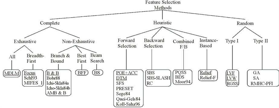
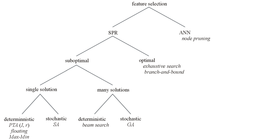
Feature selection (also known as subset selection) is a process commonly used in machine learning, wherein a subset of the features available from the data is selected for application of a learning algorithm. The best subset contains the least number of dimensions that most contribute to accuracy; the remaining and unimportant dimensions are disregarded. This is an important stage of pre-processing and is one of the two ways of avoiding the curse of dimensionality (the other one is feature extraction). From one aspect of view, feature selection method is categorized as complete, heuristic, and random methods (Figure 1). The close to optimal space search and the ease of integration with other methods, have made heuristic methods desirable. From a different point of view, feature selection is categorized as node pruning and statistical pattern recognition (SPR) (Figure 2). If these two categorizations are considered together, combination of Artificial Neural Network (ANN) and backward feature selection could be considered as a powerful solution. However, generally ANN has a major disadvantage which is stopping at the local minima instead of global minimum. Especially when backward feature selection is used, more local minima is added when removing features which leads to less accuracy. To solve this problem and avoid local minima ANN topology can be improved using complexification [1] .
Complexification in evolutionary computation (EC) refers to expanding the dimensionality of the search space while preserving the values of the majority of dimensions. In other words, complexification elaborates on the existing strategy by adding new structure without changing the existing representation. Thus, the strategy does not only become different, but the number of possible responses to situations can generate increases.
In EC domain of NeuroEvolution (i.e. evolving neural networks), complexification means adding nodes and connections to already-functioning neural networks and this is the main idea behind NEAT [2] . NEAT begins by evolving networks without any hidden nodes. Over many generations, new hidden nodes and connections are added, complexifying the space of potential solutions. In this way, more complex strategies elaborate on simpler strategies, focusing search on solutions that are likely to maintain existing capabilities.
Expanding the length of the size of the genome has been found effective in previous works [3] [4] . NEAT advances this idea by making it possible to search a wide range of increasingly complex network topologies simultaneously. This process is based on three technical components. First, it keeps track of which genes match up with which others among differently sized genomes throughout evolution. Second part is speciation of the population so that solutions of differing complexity can exist independently. The last part is starting the evolution with a uniform population of small networks. These components work together in complexify solutions as part of the evolutionary process.
In this paper, the effort was made to evaluate the implementation of NEAT for feature selection applications. The arrangement of the rest of the paper is as follows:
Section two is devoted to the required background, evolutionary neurons and derivation of complexificationare discussed as the infrastructures of the NEAT network. Section three discusses the NEAT method and section four presents the feature selection methods used in this paper and the results. Finally, the last section concludes the paper and talks about the future work.
2. Background
In order to get familiar with the concepts of this paper, it is essential to start with a short overview on derivations of complexification and continue with NEAT topology and functionality.
Derivations of Complexification
Mutation in nature results in optimization of the existing structures and occasionally addition of the genes to the new genome which results in function complexification and optimization. In distinct kinds of mutation called gene duplication, one or more parental genes are copied into an offspring’s genome at least once. As a result, the offspring has duplicated genes pointing to the same proteins. The offspring then has redundant genes expressing the same proteins. Gene duplication has been responsible for key innovations in overall body morphology over the course of natural evolution [5] [6] . Duplication creates more points at which mutations can occur. Gene duplication is a possible explanation of how natural evolution indeed expanded the size of genomes throughout evolution, and provides inspiration for adding new genes to artificial genomes as well.
Koza [7] invented a method based on gene duplication in 1995. In his algorithm, the entire function in the genetic program can be duplicated due to a single mutation followed by alternation through further mutations. For an expanding evolutionary neural network, this process will be full-fledged by adding new neuron and connections to the network. In order to implement this idea in artificial evolutionary systems, we are faced with two major challenges. First, when evolving in evolutionary neural network, different size and shape networks are faced; secondly, even the topologies might be different causing lost of information when doing crossover. For instance, depending on when a new structure is added, the same gene may exist at different positions, or conversely, different genes may exist at the same position. Thus, artificial crossover may disrupt evolved topologies through misalignment. Second, it is hard to find the innovative solution due to the variable-length genomes. Optimizing many genes takes longer than optimizing only a few, meaning that more complex networks may be eliminated from the population before they have a sufficient opportunity to be optimized.
In case of variable-length genomes, there is a natural mechanism for aligning genes with the counterpart during crossover which was addressed by E. coli [8] [9] . In this mechanism, which is called synapsis, a special protein called RecA takes a single strand of DNA and aligns it with another strand at genes that express the same traits, called homologous genes. Speciation governs innovations in nature. Entries with significantly similar gnomes mate since they belong to the same species. If any organism could mate with any other, organisms with initially larger, less-fit genomes, would be forced to compete for mates with their simpler, more fit counterparts. As a result, the larger, more innovative genomes would fail to produce offspring and disappear from the population.
In contrast, in a speciated population, organisms with larger genomes compete for mates among their own species instead of with the population at large. That way, organisms that may initially have lower fitness than the general population still have a chance to reproduce, giving novel concepts a chance to realize their potential without being prematurely eliminated. Because of speciation benefits, a variety of speciation methods have been employed in EC [10] [11] .
It turns out complexification is also possible in evolutionary computation if abstractions of synapsis and speciation are made part of the genetic algorithm. The NEAT method is an implementation of this idea: The genome is complexified by adding new genes which in turn encode new structure in the phenotype, as in biological evolution. Complexification is especially powerful in open-ended domains where the goal is to continually generate more sophisticated strategies.
3. NeuroEvolution of Augmenting Topologies (NEAT)
In this section, effort was made to address the working scenario of the NEAT. It depicts general description of the genetic encoding and the fundamental of NEAT.
The combination of the usual search for appropriate network weights with complexification of the network structure is the two major concepts on which NEAT is based. First of all NEAT method gives us knowledge about kind of genetic representation which allows disparate topologies to cross over in a significant way. Historical marking to line up genes with the same origin is used. Also, a way to protect the topological innovation, that needs a few generations to optimize, is considered so that the innovation does not vanish from the population prematurely. In this work, each innovation was separated into different species. Also, NEAT provide us with a way to minimize the topologies throughout evolution in order to find the most efficient solution. In this paper, this goal was achieved by starting from a minimal structure and adding nodes and connections incrementally.
Genetic Encoding
Genetic encoding used for NEAT is designed in a way to allow corresponding genes to be easily combined in a case when two genes crossover during mating. Genomes are linear representations of network connectivity and include the information of the two node genes being connected. Nodegenes, themselves, consist of the list of inputs, hidden nodes and possibly connected outputs. Each connection gene represents the in-node, the out-node, the weight of the connection, enable width (even if the connection gene does not exist) and innovation number which will be discussed later. Mutation in NEAT enables us to change both connection weights and network structures. Connection weights mutate (in any system) with any connection (even perturbed) at each generation.
Structural mutations can be grouped in two as illustrated in Figure 3. Fundamentally each mutation grows the genome size by adding genes. In add connection mutation method, a new connection gene is added to connect two previously unconnected nodes with a random weight. In add node mutation, the old connection is split and the new node replaces the old connection. So the old connection will be disabled and instead the two new connections will be added to the genome. The weight of the new connection which is connected to the new node is initially one and the new connection leading out receives the same weight as the old connection. This method minimizes the initial effects of the mutation. The new nonlinearity in the connection changes the function slightly, but new nodes can be immediately integrated into the network, as opposed to adding extraneous structure that would have to be evolved into the network later. As a conclusion, the network has some time to be optimized through its new structure [12] .
By applying mutation the genomes in NEAT will grow larger, resulting in genomes of varying size with different connections at the same positions. Allowing genomes to grow unbounded will result in the most complex of the competing convention problem including numerous different topologies and weight combinations. The necessity of using NEAT to overcome this problem is going to be explained later on.
4. NEAT for Feature Selection
In this section, the implementation of the NEAT algorithm for feature selection is described and its performance is evaluated against Multi-Layer Perceptron (MLP) networks.
In the case of artificial neural networks (ANN), direct estimation methods are preferred because of the computational complexity of training an ANN. Inside this category we can perform another classification based on the analysis of the training set [13] . There are many different methods to define feature selection on a trained
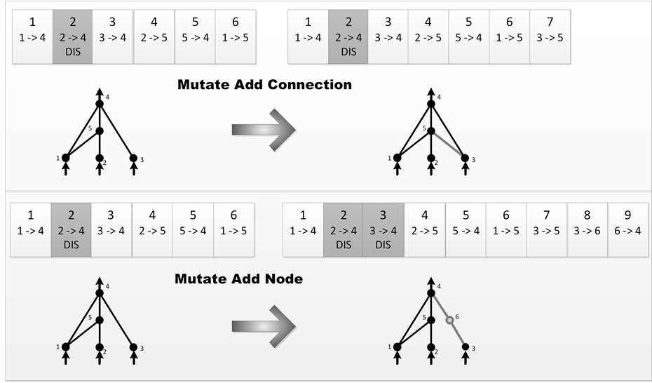
Figure 3. The two types of structural mutation in NEAT.
neural network. Some of them are specifically based on the analysis of a trained feed forward network and the others are general methods which have the ability of doing feature selection in all kinds of trained networks.
For example, according to the definition of relevance of an input unit,  , in a feed forward neural network input Ii is considered more important if its relevance
  is larger. Also relevance
  of a weight Wij connected between the input units i and the hidden unit j is defined. The relation between
  and
and  is shown in Equation (1), where Nh is the number of hidden units.
 (1)
(1)
The criteria for defining weight relevance are varied. Some of them are based on direct weight magnitude. As an example, the criterion proposed by Belue [14] is reflected in Equation (2).
 (2)
(2)
Other criteria of weight relevance, introduced by Tekto [15] , is based on an estimation of the change in the MSE (Mean Square Error), when setting the weigh to 0. Another method proposed by Utans [16] focuses on the MSE, and calculates its increment when substituting an input for its mean value. One input is considered more relevant if the increment of MSE is higher.
According to M. F. Redondo and C. H. Espinosa [17] the best method for feature selection is using a trained network proposed by Utans [16] . As Utans using MSE and this value is not feasible for NEAT, in this paper we propose another feature selection method based on Utans. Assume we have p instances and each instance has n features  and notation for features of jth instance is
 . Our method (ACCUTANS) contains following steps:
1) Train NEAT with all features 
2) Calculate mean value of feature  using Formula (3):
 (3)
(3)
3) For , in all samples, replace value of kth feature with
  and calculate confusion matrix (Table 1) for each feature separately. In each step calculate accuracy (Acc) after replacing feature k with
  using below formula:
 (4)
(4)
4) A feature is considered more relevant if the accuracy after replacement is lower.
5) Remove feature with the lowest accuracy and repeat the above steps until accuracy changes significantly.
5. Results
In order to empirically evaluate NEAT for feature selection as implemented by our approximate algorithm, we ran a number of experiments on both artificial and real-world data. These datasets include: SPEC Heart, Breast cancer, Pima Indians Diabetes, Soybean (large), and LED all from the UCI repository of machine learning databases [18] . They either contain many features and good candidates for feature selection or they are well understood in terms of feature relevance. For each dataset we train NEAT network with population sizes of {100, 150, 200, 250} and number of input nodes of 2 as initial values. The probability of addinga node in mutation is set to {0.01, 0.02, 0.03, 0.04, 0.05} for five different runs, and the probability of adding connection is set to 0.05. The network is compared against a 2-layer perceptron neural network with 25 and 50 neurons in each layer for two different runs. The classification is applied to five different datasets, SPEC Heart, Breast cancer, Pima Indians Diabetes, Soybean (large), and LED all from the UCI repository of machine learning databases [18] . These datasets are detailed in Table 2. They have been selected because they are well understood in terms of feature relevance. To improve accuracy of training in case of datasets with less number of instances, 10-fold cross-validation is applied.
The first dataset is SPEC Heart describes diagnosing of cardiac Single Proton Emission Computed Tomography (SPECT) images. Each of the patients is classified into two categories: normal and abnormal. The database of 267 SPECT image sets (patients) was processed to extract features that summarize the original SPECT images. As a result, 22 continuous feature patterns were created for each patient then these patterns were processed to obtain 16 feature patterns. According to Table 3, using NEAT and UTANS eight features could be reduced (K shows number of removed features) without losing accuracy significantly. Although MLP with 50 neurons has better performance for this dataset with all the features included, but after removing features, NEAT works better on this dataset.
The second dataset is related to breast cancer with ten features and the training set size of 699. This case is much similar to the first case where MLP-50 has slightly better performance before feature removal, but after removing only two features NEAT has significantly better performance. This illustrates NEAT supremacy in better adjusting after removing irrelevant features from the dataset.
The third dataset utilized in our evaluation is Pima with 789 data, eight features, and two classes. In this case NEAT not only has better performance to get trained but also after removing two less relevant features, NEAT still is a better model to train on Pime dataset.
Soybean (large) is the fourth dataset used in our evaluation, and with 35 features, this is more complex than previous three datasets. As can be seen in Table 3, there is significant improvement in accuracy of training

Table 1. Confusion matrix.
Table 2. Datasets used and their properties. “CV” indicates 10-fold cross-validation.
Table 3. Comparison of selecting features using NEAT and UTANS against MLP where MLP-25 is MLP with 25 neurons in each layer, MLP-50 is MLP with 50 neurons in each layer and K is number of removed features.
datasets after removing irrelevant features in NEAT compared to the other methods. This outcome supports our hypotheses in superiority of our method in accurately removing irrelevant features.
Finally, the last dataset, LED, is an artificially made dataset with randomly inserted noise. Because of the random noise, training for this data set is more complicated compared to the other data sets as this noise may lead to increased number of local minimums.
As it is illustrated in Table 3, before feature removal, NEAT trains vastly better than MLP. It can be shown that in case of having many local minimums, NEAT is capable of generating of more accurate results. Furthermore, after removing irrelevant features, NEAT still poses better performance compared to other methods. This is very important because it shows how accurately NEAT can remove irrelevant features. Also based on the results, after removing two features, the decrease of accuracy is legible which represents the power of NEAT-base model in perfectly diagnosing noisy features.
Table 4 illustrates the average accuracy for each method and dataset. It can be seen in almost all the data sets that NEAT using UTANS has the best performance. Although in SPEC Heart and Breast Cancer datasets MLP- 50 has better performance prior to feature removal, but after removing irrelevant features, NEAT performs better than the other methods.
For Pima dataset, the accuracy of NEAT is only slightly higher than the other methods. The reason is that for this specific data set, all the methods listed in the table have good performances. However, in case of Soybean (large) and LED data sets, the result of NEAT is significantly better than the other methods. These two datasets have two main differences compared to the other datasets. Soybean (large) has more features than the other datasets, and consecutively, training and selecting irrelevant features for this dataset is more demanding. In case of LED data set, the high level of the randomness increases the difficulty level for feature reduction. In both cases, existence of local minimums leads to more challenge for MLP to train and extract irrelevant features. In contrast and according to the results, NEAT using UTANS significantly increases accuracy of selecting irrelevant features.
6. Conclusions
In this paper, a new model for optimal feature selection based on NEAT and UTANS feature elimination has been presented and evaluated. The main drawback of backward feature selection methods based on ANN is that the local minima affect their accuracy negatively. Moreover by removing a feature using backward feature selection more local minima may be added to solution space. This problem can be more significant in datasets with more features such as Soybean (large) or in datasets with some parameters of randomness, such as LED. However, in small datasets this difference may not be as significant.
From these five dataset all except LED are real-world data. LED is artificially generated data with random noise insertion. As illustrated in Table 3 the accuracy of the output, using NEAT and UTANS for SPEC Heart, Breast Cancer, Soybean (large), and LED was improved. Most importantly, however, is the fact that in many datasets our feature selection algorithm can make reduction in the feature space and consequently improve classification performance. This is true especially for SPEC Heart and LED, where MLP does not improve the performance in any scenario.
Table 4. Comparison of average accuracy between NEAT.
There are many open areas ahead of this work. The implemented feature selection method through the NEAT is based on backward feature selection. Pervious works show forward feature selection can be as effective as backward and therefore worth investigating. Also both methods can be utilized at the same time to improve accuracy. Finally, this method may be compared against some other more recent techniques such as Random Forest and Adaboost in large scale datasets.
References
- Lam, H.K., Ling, S.H., Tam, P.K.S. and Leung, F.H.F. (2003) Tuning of the Structure and Parameters of a Neural Network Using an Improved Genetic Algorithm. IEEE Transactions on Neural Networks, 14, 79-88.
- Stanley, K.O. and Miikkulainen, R. (2002) The Dominance Tournament Method of Monitoring Progress in Coevolution. Proceedings of the Bird of a Feather Workshops, Genetic and Evolutionary Computation Conference, AAAI, New York, 242-248.
- Cliff, D. (1993) Explorations in Evolutionary Robotics. Adaptive Behavior, 2, 73-110. http://dx.doi.org/10.1177/105971239300200104
- Harvey, I. (1993) The Artificial Evolution of Adaptive Behavior. Ph.D. Thesis, University of Sussex, Brighton.
- Force, A., Yan, Y.L., Joly, L., Amemiya, C., Fritz, A., Ho, R.K., Langeland, J., Prince, V., Wang, Y.L., Westerfield, M., Ekker, M., Postlethwait, J.H. and Amores, A. (1998) Zebrafish HOX Clusters and Vertebrate Genome Evolution. Science, 282, 1711-1714. http://dx.doi.org/10.1126/science.282.5394.1711
- Lynch, M., Bryan Pickett, F., Amores, A., Yan, Y., Postlethwait, J. and Force, A. (1999) Preservation of Duplicate Genes by Complementary, Degenerative Mutations. Genetics Society of America, 151, 1531-1545.
- Koza, J.R. (1995) Gene Duplication to Enable Genetic Programming to Concurrently Evolve both the Architecture and Work-Performing Steps of a Computer Program. Proceedings of the 14th International Joint Conference on Artificial Intelligence, Montréal, 1995, 734-740.
- Radding, C.M. (1982) Homologous Pairing and Strand Exchange in Genetic Recombination. Annual Review of Genetics, 16, 405-437. http://dx.doi.org/10.1146/annurev.ge.16.120182.002201
- Sigal, N. and Alberts, B. (1972) Genetic Recombination: The Nature of a Crossed Strand-Exchange between Two Homologous DNA Molecules. Journal of Molecular Biology, 71, 789-793. http://dx.doi.org/10.1016/S0022-2836(72)80039-1
- Goldberg, D.E. (1987) Genetic Algorithms with Sharing for Multimodal Function Optimization. Proceedings of the 2nd International Conference on Genetic Algorithms, Pittsburg, 1987, 41-49.
- Mahfoud, S.W. (1995) Niching Methods for Genetic Algorithms. Ph.D. thesis, University of Illinois at Urbana-Champaign, Urbana.
- Stanley, K.O. and Miikkulainen, R. (2002) Evolving Neural Networks through Augmenting Topologies. The MIT Press Journals, 10, 99-127.
- Battiti, R. (1994) Using Mutual Information for Selection Features in Supervised Neural Net Learning. IEEE Transactions on Neural Networks, 5, 537-550. http://dx.doi.org/10.1109/72.298224
- Bauer Jr., K.W. and Belue, L.M. (1995) Determining Input Features for Multilayer Perceptron. Neurocomputing, 7, 111-121. http://dx.doi.org/10.1016/0925-2312(94)E0053-T
- Villa, A.E.P., Livingstone, D.J. and Tetko, L.V. (1996) Neural Network Studies. 2. Variable Selection. Journal of Chemical Information and Computer Sciences, 36, 794-803. http://dx.doi.org/10.1021/ci950204c
- Moody, J., Rehfuss, S. and Utans, J. (1995) Input Variable Selection for Neural Networks; Application to Predicting the US Business Cycle. Proceedings of IEEE/IAFE 1995 Computational Intelligence for Financial Engineering, New York City, 1995, 118-122.
- Redondo, M.F. and Espinosa, C.H. (1999) A Comparison among Feature Selection Methods Based on Trained Networks. Proceedings of the IEEE Signal Processing Society Workshop, Madison, 1999, 205-214.
- Bache, K. and Lichman, M. (2013) Machine Learning Repository. University of California, Irvine.
- Alelyani, S., Liu, H. and Tang, J. (1997) Feature Selection for Classification. Intelligent Data Analysis, 1, 131-156.
- Jain, A. and Zongker, D. (1997) Feature Selection: Evaluation, Application, and Small Sample Performance. IEEE Transactions on Machine Intelligence, 19, 153-158.