Journal of Service Science and Management
Vol.6 No.3(2013), Article ID:35509,7 pages DOI:10.4236/jssm.2013.63023
A Markov Model for Human Resources Supply Forecast Dividing the HR System into Subgroups
![]()
Mohammadia School of Engineering Rabat, Studies and Research Laboratory in Applied Mathematics (LERMA), Mohammed V University, Agdal, Morocco.
Email: rachidblh@yahoo.fr, mohamedtkiouat@gmail.com
Copyright © 2013 Rachid Belhaj, Mohamed Tkiouat. This is an open access article distributed under the Creative Commons Attribution License, which permits unrestricted use, distribution, and reproduction in any medium, provided the original work is properly cited.
Received April 17th, 2013; revised May 26th, 2013; accepted July 10th, 2013
Keywords: Manpower Planning; Forecasting; Markov Modeling
ABSTRACT
Modeling the manpower management mainly concerns the prediction of future behavior of employees. The paper presents a predictive model of numbers of employees in a hierarchical dependent-time system of human resources, incorporating subsystems that each contains grades of the same family. The proposed model is motivated by the reality of staff development which confirms that the path evolution of each employee is usually in his family of grades. That is the reason of dividing the system into subgroups and the choice of the superdiagonal transition matrix.
1. Introduction
Human Resources Planning (HRP) according to Collings [1] represents the range of philosophies, tools and techniques that any organization should deploy to monitor and manage the movement of staff, both in terms of numbers and profiles.
Traditionally, manpower planning focused on the number of employees and levels and types of skills in the organization. A typical model of the traditional manpower planning is shown in the model of Torrington et al. [2], Figure 1.
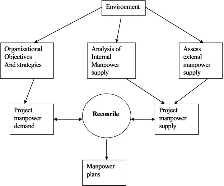
Figure 1. A model of traditional manpower planning.
In the model of Torrington the emphasis is placed on the balance between demand and supply, in order to have the right number of employees in the right place at the right time. Demand is influenced by the strategies and business objectives. Supply is projected from current employees (via calculations of expected leavers, retirements, promotions, etc.) and availability of skills in the labor market.
The demand and supply are then reconciled by considering a range of options and plans to achieve a feasible balance. Optimal recruitment and transition patterns are determined by minimizing expected discrepancies between actual states and preferred goals Mehlmann [3], Poornachandra [4].
2. The Forecast of Future Demand and Supply
2.1. The Demand Forecast
The demand forecast anticipates the future manpower that will be needed to accomplish the future functional requirements and carry out the mission of the organization. In this step, a review of staffing requirements against future functional requirements is performed.
2.2. The Prediction of Supply
The prediction of the offer according to Torrington et al. [2], is subject to how the current supply of employees will change internally. These changes are anticipated by analyzing what happened in the past, in terms of staff retention and/or movement, and extrapolating into the future to see what would happen with the same trends of the past.
In forecasting the supply of human resources, organizations must consider both internal and external supply of qualified candidates. The domestic supply of candidates is influenced by the training and the manpower development and mobility policies, promotion and retirement. In this step the Markov modeling is one of the best tools to model the manpower structure evolution.
3. State of the Art
The objective of constructing a stochastic model of the process of human resources is especially to be able to predict future numbers in the different categories of grades. The stochastic model specifies for each process, in probabilistic terms the law of change in each individual level.
Researchers used a Markov model associated or integrated to describe the change of the process in light of its historical evolution, Bartholomew [5]. Although these models are formulated in stochastic terms, they are always treated in a discreet way. The current number of individuals in a group of grades is a random variable, but the analysis proceeds by replacing each random variable by its expectation.
The concept of the Non-Homogeneous Markov Systems (NHMS) in modeling the manpower system was introduced by Vassiliou [6]. Presentations in the literature of the theory of NHMS have flourished in recent years Vassiliou and Georgiou [7], Vassiliou et al. [8].
Tsantas and Vassiliou [9] had the idea to provide a stochastic structure for the NHMS in establishing a model with an inherent stochastic mechanism. Their efforts have involved the construction of a procedure which allows the NHMS to select among several possibilities transition.
Nilakantan and Raghavendra [10] suggested a policy of proportionality of the Markov system, namely recruitment at all levels of the hierarchy (except at the lowest level) to be in strict proportion to the levels in these promotions. Another idea was presented by Georgiou and Tsantas [11] who have enriched the framework NHMS with an external state next to the original class/internal (active), it is the Augmented Mobility Model (AMM).
Dimitriou and Tsantas [12] then presented an improved model GAMM namely “the Generalized Augmented Mobility Model”, it is a time-dependent hierarchical system of (human resources) incorporating training classes and two recruitment channels: the external environment and other external auxiliary system consisting of potential candidates (who are part of a preparatory class).
Recently, new ideas were presented in the field of mathematical models for manpower planning. An interesting idea was proposed by De Feyter [13], which divides the population of the studied system into several more homogeneous subgroups. The division was based on characteristics such as: gender, number of children by individuals...etc. This provides an opportunity for a deep investigation and probably more sophisticated.
In this article we will address the problem of planning by dividing the entire heterogeneous manpower system in several homogeneous subgroups (families of the same grades) which form a partition of the entire personnel system. This simplifies the prediction of the manpower evolution, as it becomes acceptable that everyone in the same group evolves similarly. The proposed model gives a more realistic view of the manpower advancement and the development of each employee in his normal family, this model finds its motivation in the following findings:
Ÿ The consolidation of staff by grade family of the same nature (agents, technicians, executives, managers, leaders...) facilitates the prediction of the career path of each employee in his family by limiting its area of movement. Thus each family of grade will be given a special transition matrix does not interfere with the data of inaccessible grades.
Ÿ In most cases, the career of an individual in an organization is related to its level of study and diplomas while hiring. The grades to which each employee can be promoted (compatible of course with his training, skills, experience...) are limited, therefore his entire career can be known in advance and will be accomplished without many surprises.
Ÿ A fourth grade technician for example has practically zero chance of seeing one day finish his career with the rank of chief, because on the one hand the time required for the advancement from one grade to another in this example does not allow it, on the other hand those of a higher academic level are more likely to hold this position. Only by additional studies sanctioned by higher degrees (which is difficult and rare at a time) that a technician can expect to climb the ladder quickly. This example inspires us to put each employee in his normal family where he can evolve.
In the next section we begin by recalling the notations and formulas modeling the manpower planning by Markov chains, and then the object model of this section is presented with its parameters and the different formulas that characterize it to arrive to the equation that determines the structure of the projected population at any time t. The last section is reserved to a numerical application of the theoretical results of the model.
4. The Model Overview
We begin by a recalling of the notations and formulas modeling the manpower planning by Markov chains.
The stochastic modeling of the HR system; Tsantas [14] is as following:
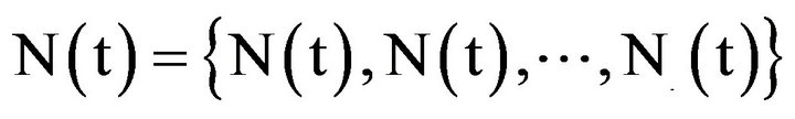
Consider a discrete time scale t = 0, 1, 2, ... and G = {1, 2, ..., k} a set of classes of a system that is supposed exclusive and exhaustive. The system state at each date t is represented by the row vector N (t) = [N1 (t), N2 (t) ... Nk (t)] of numbers of individuals in classes at the time t.
We assume that the individual transitions between classes are on a non-homogeneous Markov chain. In this model, individual movements are represented by a timedependent sub stochastic matrix.
The system of HR can be represented by a NHMS (Non-Homogeneous Markov System); Tsantas [14] defined by:
Ÿ The state of the system: N (t) = [N1 (t), N2 (t), ... Nk (t)] with:
Ÿ Ni (t): the number of individuals in class i at time t.
Ÿ N (0): the initial structure.
Ÿ {T (t)}∞t=0: a sequence indicating the total size of the system.
Ÿ P (t): the transition matrix.
Ÿ {Pk +1 (t)}∞t=0, Pi,k+1 (t) is the probability of departure of the ith individual to a hypothetical class k + 1 that shows the external environment where those leaving the system are transferred.
Ÿ {P0 (t)} t ≥ 0, a new recruit is allocated to class j with probability P0J (t) j Є G, these probabilities collected in a row vector P0 (t) is called the distribution of recruitment.
The embedded non-homogeneous Markov chain:
Let Q (t) = P (t) + P'k+1 (t) P0 (t), the matrix Q (t) is a stochastic matrix and defines what is called an embedded non-homogeneous Markov chain.
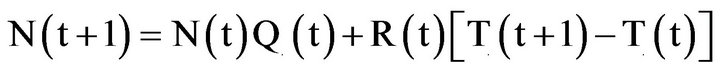
The forecasted structure of the system at the time t according to that at the time  is:
is:

5. The Proposed Model Parameters
5.1. The System
The hierarchical system of grades constituting the organization is divided into subsets Si, S = {S1, S2, S3, ..., Sn}, each subset is formed by a family of grades of the same kind, i.e. a family whose people come from the same initial training that provides the same level of study. Si is written as Si = (si1, si2, ..., sim), knowing that sij is the rank j of the family of grade i. sij are the different levels of the grade, for example for the grade of technician the levels are technician of first grade, second grade, etc.
5.2. The Subgroups of the System
A subgroup is a family of grades made by people with the same education level, experience, etc., a family of technicians will be made by the technicians of various levels (fourth grade technicians, third grade technicians, second grade technicians, first grade technicians...), and a family of leaders will be formed by people with the capacity as the holder of executive responsibility (Chief of a Bureau, Chief of a section, Project Manager, department head, division head...).
5.3. The Transition Matrix
For every subset Si is assigned a transition matrix Pi. Our system is hierarchical and it is assumed that the promotion is done only to the first next higher grade, and therefore the transition matrix will be superdiagonal. Within each family operates the movement of its staff.
5.4. The Departure
A departure vector is assigned to each family; this vector contains the proportions of people of each level who will leave the family. In our model the leavers move to the next family and to the external environment.
5.5. The Recruitment
A distribution recruitment vector is assigned to each family, the components of this vector equal to the recruitment proportion of individuals to the corresponding level. Since our Human Resources System is hierarchical the recruitment proportion in the first level of the family Si+1 comes from Si and the external environment.
5.6. The Model Parameters
Consider a discrete time scale t = 0, 1, 2 ... and S = {S1, S2, S3, ..., Sn} is a group of families of grades of a system that is supposed exclusive and exhaustive. Si = (si1, si2, si3 ..., sim) is a subset of S consisting of levels of the same family. Knowing that sij level is greater than the level si,j-1, and also the grade of Si is higher than that of Si-1, see Figure 2.
We assume that the individual transitions between classes are on a non-homogeneous Markov chain. In this
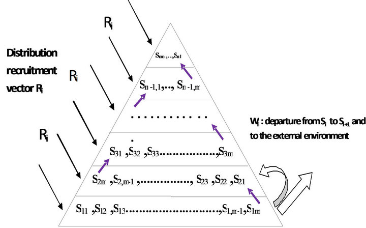
Figure 2. Model of manpower system division.
model, individual movements are represented by a timedependent sub stochastic matrix of transition probabilities.
The HR system can be represented by a NHMS (NonHomogeneous Markov System) defined by:
Ÿ The system state at each date to come t is represented by the row vector N (t) which components are the Ni (t) = [ni1 (t), ni2 (t), ..., nim (t)]. 1 ≤ i ≤n, with: nij (t): the number of individuals in the level j at the time t of the family of grades i.
Ÿ N (0): the initial structure.
Ÿ Wi (t): the departure vector of the elements of the family i.
Ÿ Ri (t): the recruitment distribution vector of the family of grade i, Ri (t) = [ri1 (t), ri2 (t), ..., rim (t)].
Ÿ {T (t)} 0 ≤ t ≤ n: the sequence indicating the total size of the system.
Ÿ Pi (t) 1 ≤ i ≤ n: the transition matrix specific to the family of grades i, it is a superdiagonal matrix.
The forecasted structure in the family i at time t +1 according to that at time t is:

Note that for a given family:
The embedded non-homogeneous Markov Chain:
Let Qi (t) = Pi (t) + w'i (t) Ri (t), the matrix Qi(t) is a stochastic matrix and defines what is called an embedded non-homogeneous Markov chain.
The forecasted structure in the family i at the time t +1 according to that at the time t is:
The forecasted structure of the system at time t + 1 according to that at time t is:
6. Numerical Example
In this section we will present an example that will illustrate the model described above. Consider a system of five families of grades S = {S1, S2, S3, S4, S5} see Table 1.
The human resources system is modeled using a Markov chain with four states for each family. The starting structure is shown in the Table 1, the target structures suits the strategic objectives of the organization (There is an assessment of the future demand for HR, taking into account the current situation, the external environment and the organization’s business plan), see Table 1.
In the Table 1 is also shown the vector of the starting

Table 1. The human resources system: S.
recruitment probabilities (you can notice that since our system is hierarchical the highest recruitment probabilities concern the first levels of the family. Inversely the highest departure probabilities are in the last levels of the family because it is logic that the employees of the family Si intend to reach the positions in the family Si+1). Pi is the transition matrix (obtained from historical data), for each family there is a transition matrix.
The transition matrices P1 to P5 (obtained from historical data) provide the proportions of employees that remain in the same position and the one that move to the next level. Since our Human Resources System is hierarchical the employees in first levels try to move up to the highest onesP1 = [0.5 0.4 0 0, 0 0.6 0.3 0, 0 0 0.5 0.2, 0 0 0 0.5];
P2 = [0.5 0.4 0 0, 0 0.6 0.3 0, 0 0 0.6 0.2, 0 0 0 0.4];
P3 = [0.5 0.4 0 0, 0 0.6 0.3 0, 0 0 0.6 0.2, 0 0 0 0.4];
P4 = [0.65 0.325 0 0, 0 0.5 0.375 0, 0 0 0.5 0.375, 0 0 0 0.275];
P5 = [0.6 0.375 0 0, 0 0.75 0.225 0, 0 0 0.6 0.275, 0 0 0 0.175].
The total structures for all Si during the planning horizon of 10 years are in the Table 2.
The simulation with Matlab (see an example of the Matlab code here after) returns a matrix A (10 × 4), in the first line is stored the initial structure, the row i gives the structure of the family at time i (1 ≤ i ≤ 10). The first column shows the evolution in numbers of level 1, the other columns stand the same for the other levels of the family, see matrices Ai and graphical representations in the Figure 3.
Example of the Matlab code (Family S1):
p = [0.5 0.4 0 0; 0 0.6 0.3 0; 0 0 0.5 0.2; 0 0 0 0.5]% The transition matrix x = [20; 16; 14; 12]% The starting structure y = [0.5 0.25 0.15 0.1]% The recruitment probabilities vector t = [62 70 76 80 86 92 100 114 120 130]% The total structure size of S1 for 10 years k = [0.1; 0.1; 0.3; 0.5]% The departure probabilities vector t = 10 % The planification horizon A = zeros (t,4)% The states matrix A(1, :) = X B=zeros(t,4)
B(1, :)=y for n = 1:(t − 1)
Q = P+[K * B( n,:)]
A(n + 1, :) = A(n, :) * Q + [ T(n + 1) − T(n)] * B( n, :)
B(n + 1, :)=A(n + 1, :)/T(n + 1)
end v = A (:,1) w = A (:,2) z = A(:,3) s = A (:,4) plot ([1:10]', [v'; w'; z'; s'])
The Table 3 shows the results of the evolution of the families S1 to S5.
Reading and interpreting the results of the Table 3:
The results table shows the evolution of the staff number of the four levels constituting the families S1, S2, S3, S4, and S5. There are differences observed between the structure at the planning horizon and the target structure.
The results Table 4 shows the levels of grades that are in surplus or in shortfall of the four levels constituting each family.
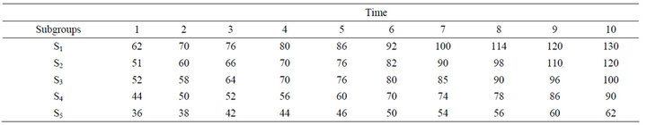
Table 2. The total structures size for all Si during the planning horizon of 10 years.
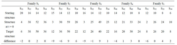
Table 3. Results and differences between the structure at t = 0 and the target structure.


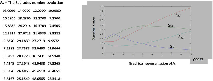
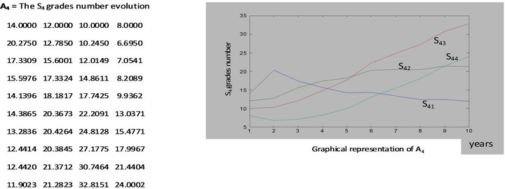
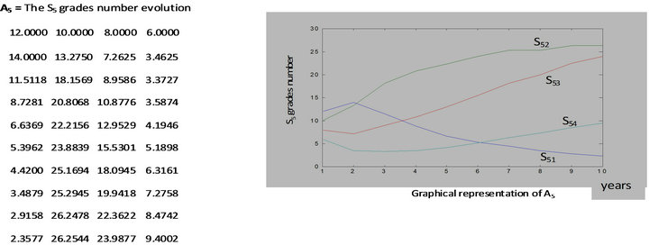
Figure 3. Results and graphical representation of the evolution of all Si.
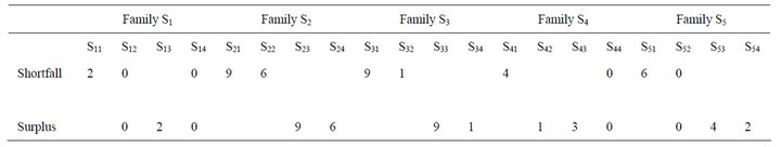
Table 4. Shortfalls and surpluses found between the structure at t = 0 and the target structure.
Analysis of the Family S1
In this family we need two employees in S11 to meet the target structure, while in S13 we have two employees in surplus. The numbers in S12 and S14 coincide with the target numbers.
The same analysis is to be done for the other families.
After the analysis of the differences between the numbers required in the target structure (the demand) and the numbers forecasted at t = 10 by the proposed model (the supply), the Human Resources Planning reconciles the two and indicates how the shortfall can be met and how the surplus is to be shed.
The plan will consist of the traditional methods of dealing with the shortfall or surplus which will involve for example a recruitment or disposal plan.
7. Conclusion and Perspective
In this paper we proposed a model of human resource management system that divides the staff into homogeneous subgroups; the elements of each subgroup belong to the same family of grades. Our system is hierarchical and it was assumed that the promotion is done only to the first next higher grade, and so we proposed a superdiagonal transition matrix.
The motivation of this model is that for each employee of the organization the promotion possibilities are limited, and therefore it is more appropriate to put each individual into his normal family where he will evolve. A numerical model is presented; it gives the gaps between the management expectations and the forecasting results. These will be studied by managers to choose the possible reconciliation plans. An opening view of this research will be the division of the manpower system by subgroups of competences; the objective will be to ensure the availability of skills (that may only be acquired within the organization).
REFERENCES
- D. G. Collings and G. Wood, “Human Resource Management, a Critical Approach,” Routledge, London, 2009.
- D. Torrington, L. Hall and S. Taylor, “Human Resource Management,” 6th Edition, Financial Times Prentice Hall, Harlow, 2005.
- A. Mehlmann, “An Approach to Optimal Recruitment and Transition Strategies for Manpower Systems Using Dynamic Programming,” Journal of the Operational Research Society, Vol. 31, No. 11, 1980, pp. 1009-1015.
- R. Poornachandra, “A Dynamic Programming Approach to Determine Optimal Manpower Recruitment Policies,” Journal of the Operational Research Society, Vol. 41, No. 10, 1990, pp. 983-988.
- D. J. Bartholomew, “Stochastic Models for Social Processes,” 3rd Edition, Wiley, Chichester, 1982.
- P. C. G. Vassiliou, “Asymptotic Behavior of Markov Systems,” Journal of Applied Probability, Vol. 19, No. 4, 1982, pp. 851-857. doi:10.2307/3213839
- P. C. G. Vassiliou and A. C. Georgiou, “Asymptotically Attainable Structures in Non-Homogeneous Markov Systems,” Operations Research, Vol. 38, No. 3, 1990, pp. 537-545. doi:10.1287/opre.38.3.537
- P. C. G. Vassiliou, A. C. Georgiou and N. Tsantas, “Control of Asymptotic Variability in Non-Homogeneous Markov Systems,” Journal of Applied Probability, Vol. 27, No. 4, 1990, pp. 756-766. doi:10.2307/3214820
- N. Tsantas and P. C. G. Vassiliou, “The Non-Homogeneous Markov System in a Stochastic Environment,” Journal of Applied Probability, Vol. 30, 1993, pp. 285- 301. doi:10.2307/3214839
- K. Nilakantan and B. G. Raghavendra, “Control Aspects In Proportionality Markov Manpower Systems,” Applied Mathematical Modeling, Vol. 29, No. 1, 2004, pp. 85- 116. doi:10.1016/j.apm.2004.04.003
- A. C. Georgiou and N. Tsantas, “Modeling Recruitment Training in Mathematical Human Resource Planning,” Applied Stochastic Models in Business And Industry, Vol. 18, No. 1, 2002, pp. 53-74. doi:10.1002/asmb.454
- V. A. Dimitriou and N. Tsantas, “Prospective Control in an Enhanced Manpower Planning Model,” Applied Mabthematics and Computation, Vol. 215, No. 3, 2009, pp. 995-1014.
- T. De Feyter, “Modeling Heterogeneity in Manpower Planning: Dividing the Personnel System into More Homogeneous Subgroups,” Applied Stochastic Models in Business and Industry, Vol. 22, No. 4, 2006, pp. 321-334. doi:10.1002/asmb.619
- N. Tsantas, “Stochastic Analysis of a Non-Homogeneous Markov System,” European Journal of Operational Research, Vol. 85, No. 3, 1995, pp. 670-685. doi:10.1016/0377-2217(93)E0365-5