Journal of Service Science and Management
Vol.5 No.3(2012), Article ID:22447,8 pages DOI:10.4236/jssm.2012.53029
Efficient Routing of Emergency Vehicles under Uncertain Urban Traffic Conditions
![]()
Department of Management, Bar-Ilan University, Ramat Gan, Israel.
Email: amir.elalouf@biu.ac.il
Received May 22nd, 2012; revised June 20th, 2012; accepted July 2nd, 2012
Keywords: Fast routing algorithm; FPTAS; Dynamic programming
ABSTRACT
Emergency-vehicle drivers who aim to reach their destinations through the fastest possible routes cannot rely solely on expected average travel times. Instead, the drivers should combine this travel-time information with the characteristics of data variation and then select the best or optimal route. The problem can be formulated on a graph in which the origin point and destination point are given. To each arc in the graph a random variable is assigned, characterized by the expected time to traverse the arc and the variance of that time. The problem is then to minimize the total origin-destination expected time, subject to the constraint that the variance of the travel time does not exceed a given threshold. This paper proposes an exact pseudo-polynomial algorithm and an ε-approximation algorithm (so-called FPTAS) for this problem. The model and algorithms were tested using real-life data of travel times under uncertain urban traffic conditions and demonstrated favorable computational results.
1. Introduction
The public’s concern for safety and improving quality of life has generated a need for improved service of numerous public-safety and transportation agencies. An important challenge in this regard is to improve transportation system management for emergency response.
Minimization of emergency response time is a key focus in endeavors to improve emergency transport systems. A rapid response to an emergency situation can prevent or minimize adverse outcomes such as fatalities or the loss of property. In many cases, emergency vehicles (e.g., medical ambulances, police and security cars, fire and rescue vehicles, hazardous materials trucks, and gas/ electricity repair vehicles) are exempt from conventional traffic laws so that they may reach their destinations as quickly as possible; for example, they may be permitted to drive through red lights or exceed the speed limit.
Efficient routing under uncertain traffic conditions can improve the performance of intelligent transportation systems, wherein real-time traffic information is available at emergency dispatch centers. This research aims to develop and enhance a real-time emergency response system that uses real-time travel time information to assist the dispatchers of emergency vehicles in assigning the vehicles to optimal routes. To this end, this paper proposes a mathematical model for a decision-making process in real-time route dispatching. The model is formulated as a constrained shortest-path problem that can help the dispatcher to make decisions. The problem is stochastic path planning since, in contrast to standard deterministic routing problem, it takes traffic variability into account. In addition, the computational efficiency (algorithm complexity) of the process is examined, because this computational time has a major effect on the model’s applicability in real-time situations.
The dispatching model proposed herein uses a dynamicprogramming shortest-path algorithm as the basis for a fully polynomial time approximation scheme (FPTAS). Although a number of routing models have been developed previously, the current model is substantially more flexible, incorporating a joint analysis of the expected route time and its variance. The model and algorithms were tested using real-life data of travel time under uncertain urban traffic conditions and demonstrated favorable computational results.
2. Literature Review
Emergency vehicle routing (EVR) has been an attractive subject for operations researchers for many years. Most studies on EVR systems focus on location, fleet size, and operations performance. The majority of EVR mathematical models can be categorized into the following groups:
Group one: Location of emergency vehicle stations or individual emergency vehicles within a region, subject to some performance criteria such as response time [1];
Group two: Determination of the minimum number of emergency vehicles required to cover a given area;
Group three: Dispatching strategies and their influence on performance results and services for emergency victims.
Work on emergency vehicle dispatching has generally involved the use of three approaches: queuing, mathematical programming, and dynamic programming (DP). Among studies using queuing methods, Larson [2,3] used a hypercube queuing model as a tool for facility location and redistricting in urban emergency services. Yet the ability to develop analytical methods (mathematical programming and queuing models) for EVR systems is rather limited, because even sophisticated analytical models cannot solve real-world problems under uncertain traffic data.
Cooke and Halsey [4] were the first to deal with timedependent shortest path algorithms. Their algorithm is based on Bellman’s principle of optimality and dynamic programming. Starting from the destination node, the algorithm calculates the path operating backwards. Ziliaskopoulos and Mahmassani [5] extended Cooke and Halsey’s algorithm to calculate the time-dependent shortest paths from all nodes in a network to a given destination node over a given time horizon in a network with timedependent arc costs. Goldberg and Paz [6] formulated an optimization model that allowed for stochastic travel times, unequal emergency vehicle utilizations, various call types, and service times that depend on call location. Ben-Akiva et al. [7] have shown that the static model outperforms the dynamic traffic assignment model for shorter prediction horizons. Hadas and Ceder [8] suggest a stochastic model for EVR under uncertainty that yields a set of paths and determines the probability that a given path is the shortest. The EVR algorithm proposed herein uses a combinatorial enumeration of prospective routes in combination with a simulation of several candidate shortest paths.
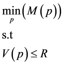
3. Problem Formulation
The problem framework is based on a computational network composed of a graph (possibly cyclic), G = (N,A), with a set N of nodes, a set A of arcs, a start node s = 1, and a destination node t = n. The term tij, denoting the time to traverse arc (i,j) in G, is a random variable characterized by two parameters: mij—the expected time, and vij the variance. |A| = h, and |N| = n. The parameters mij are assumed to be integers. A path p is called feasible if the variance of the time to traverse the path is at most R, where R is a given threshold. The problem is to find a feasible path with minimum expected time.
Mathematical Form
Problem input: G(N,A)—a given graph.
For any arc (i,j) A, two parameters are given: mij— the expected time; vij—the variance.
M(p) denotes the expected time to traverse path p;

V(p) denotes the variance of the time it takes to traverse path p. All tij are assumed to be independent random variables and therefore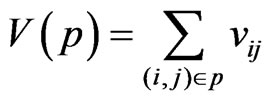 .
.
In a mathematical form the problem is to find a path p such that:
4. Exact Algorithm: Dynamic Programming
This section introduces an exact DP algorithm. Since mij are assumed to be integers, DP is a pseudo-polynomial algorithm. As a result, if mij is bounded, DP is polynomial.
Let us associate with each path p a pair (M, V), where M = M(p) is the expected time to traverse path p, and, correspondingly, V = V(p) is the variance of the time to traverse p. Sets S(k) of pairs (M, V) are arranged in increasing order of M-values, so that every pair in S(k) corresponds to a path from node s to a node k. In order to restore the path corresponding to a pair (M, V), each pair is assigned a predecessor pair, and then standard backtracking can be used.
If there are two pairs in S(k), (M1,V1) and (M2,V2) such that M1 ≤ M2 and V1 ≤ V2, then the pair (M2, V2) is called dominated and may be discarded. Let UB be the upper bound of the total expected time for the optimal path. For instance, UB can be set to . The detailed polynomial time DP algorithm is presented in Figure 1.
Proposition 1. The complexity of the DP algorithm (Algorithm 1) is O(hnUB).
Proof: Since the times are integers and dominated pairs are discarded, there are at most UB pairs in sets W and S(k). Furthermore, construction of W in lines 9 - 11 requires O(UB) elementary operations, since W is constructed from a single S(k). Merging the sorted sets W and S(k), in line 12, as well as discarding all the dominated pairs, is done in linear time (in the number of pairs, which is at most UB). In Step 2, lines 5 - 14 have two nested loops, where the first begins at line 6 and the second at line 7. These two loops go over all the arcs n − 1 times, so that in total, there are O(hn) iterations of lines 11 - 13. Thus, the total complexity of Algorithm 1 is O(hnUB).
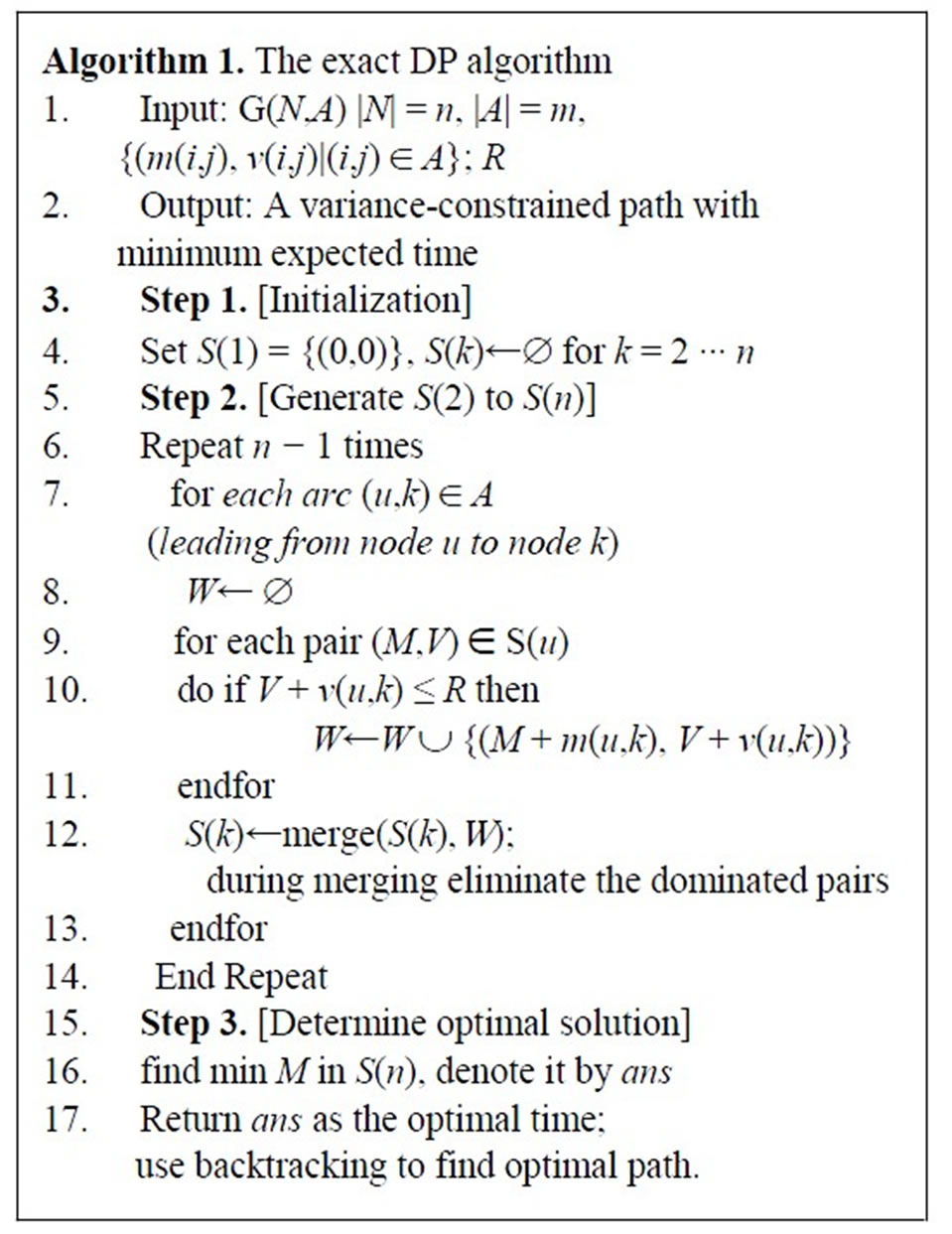
Figure 1. The exact pseudo-polynomial DP algorithm.
5. Fully Polynomial Time Approximation Scheme
5.1. General Description of the FPTAS
Our approach for constructing an FPTAS follows a socalled interval partitioning computational scheme. The interval partitioning technique was originally proposed by Sahni [9] for the knapsack problem and was later improved by Gens and Levner [10] and by Levner et al. [11] and Elalouf et al. [12]. The FPTAS in this paper consists of three main stages:
Stage A: Find a preliminary lower bound LB and an upper bound UB on the optimal path’s expected time such that UB/LB ≤ n.
Stage B: Find improved lower and upper bounds such that UB/LB ≤ 2.
Stage C: Partition the interval [LB,UB] into n/ε equal subintervals, delete sufficiently close solutions in the subintervals, and then find an ε-approximation solution using full enumeration of the “representatives” (taking only one “representative” from each subinterval).
This technique is similar to that presented by the author at the conference EOMAS-2011 and published in the conference proceedings [12]. Notice, however, that the present paper addresses another type of problem. Specifically, the underlying graph G is allowed to have cycles, and, in addition, the problem under consideration is a problem of minimizing, rather than maximizing, the objective function. As a result, the new algorithm has a different complexity.
5.2. Stage A: Finding Preliminary Lower and Upper Bounds
The following greedy technique is applied: Let A = {a1, a2, ∙∙∙, am} be the set of arcs in G(N,A). Denote graph G'(N',A') with the same set of nodes, N' = N, and the set of arcs . To define A', a binary variable, xai is used. If xai = 1 then ai
  A’; otherwise ai
  A’. The arcs in G are ordered according to their non-decreasing expected time values:
 , and are initialized at
 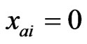 for any i = 1, ∙∙∙, h (i.e., the initial G’ is a graph with no arcs). Then the xai s are iteratively set at
  and each arc is added to the graph until a path is obtained from the source to the destination that satisfies the constraint. If all xai = 1 but such a path cannot be found, there is no feasible solution. Let xk be the last variable set to 1 in the above procedure. Then set
 . Obviously, the optimal total travel time (denoted by OPT) must lie between m0 and nm0. In cases where the OPT equals zero, the above greedy procedure in Stage A finds the exact optimal solution (i.e., a path of zero duration); therefore, Stages B and C are not required.
Complexity of Stage A. Sorting the arcs is done in O(h log h). Each check of whether the graph G has a feasible path on a selected set of arcs requires O(n2) time [13]. The total number of checks is O(logh) if a binary search is performed in the interval [1, h]. Thus, the complexity of Stage A here is O(n2logh).
5.3. Stage B: Finding Improved Bounds
This stage has two building blocks: a test procedure, denoted Test (w,ε), and a narrowing procedure denoted BOUNDS that uses Test (w,ε) as a sub-procedure.
5.3.1. Test Procedure (Test(w,ε))
Test(w,ε) is a parametric dynamic-programming type algorithm that has the following property: given positive parameters w and ε, it either reports that the minimum possible expected travel time M* ≤ w, or, otherwise, reports that M* ≥ w(1 − ε).
Test(w,ε) will be repeatedly applied as a sub-procedure in the algorithm BOUNDS below to narrow the gap between UB and LB until UB/LB ≤ 2.
Associate with each path p a pair (M,V), where M = M(p) is the path expected travel time, and, correspondingly, V = V(p), the variance of path time. Sets S(k) of pairs (M,V) are arranged in increasing order of M-values so that every pair in S(k) corresponds to a path from the start node s to a node k. As in DP, the dominated pairs in all S(k) sets are deleted.
In addition to dominated pairs, the δ-close pairs are deleted as follows: Given a δ, if there are two pairs in S(k), (M1, V1) and (M2, V2), such that 0 ≤ M2 – M1 ≤ δ, then the pairs are called δ-close. The δ-close pairs are discarded from set S(k) according to the following procedure:
1) Let w be a given parameter satisfying LB ≤ w ≤ UB. In each S(k), partition the interval [0,w] into  equal subintervals of size no greater than δ = εw/n;
2) If more than one pair from S(k) falls into any one of the above subintervals, discard all such δ-close pairs, leaving only one representative pair in each subinterval, namely the pair with the smallest (in this subinterval) V-coordinate.
3) A pair with (M,V) with M > w (called w-redundant) may be discarded.
The algorithm for Test(w,ε) is presented in Figure 2.
Proposition 2. The complexity of Test(w,ε) is O(hn2/ε)Proof: Since the subinterval length is δ = εw/n, there are O(n/ε) subintervals in interval [0,w]. Therefore there are O(n/ε) representative pairs in sets W and S(k). Further, constructing each W in lines 10 - 12 requires O(n/ε) elementary operations. Merging the sorted sets W and S(k), in line 13, as well as discarding all the dominated pairs, is done in linear time (in the number of pairs, which is O(n/ε)). In Step 2 the algorithm goes over all the arcs n-1 times, so that in total, there are O(nh) iterations of lines 10 - 12. Thus, the total complexity of Algorithm 2 is O(hn2/ε).

Figure 2. The testing procedure test (v, ε).
5.3.2. The Narrowing Procedure (BOUNDS)
The narrowing procedure presented in this section (Figure 3) is adapted from the procedure suggested by Ergun et al. [14] for solving the restricted shortest path. Namely, when Test(w,ε) runs, the ε value is chosen as a function of UB/LB, and this value is updated from iteration to iteration. To distinguish the allowable error (ε) in the FPAS from the iteratively changing error in the testing procedure, the latter is denoted as θ. The complexity of BOUNDS is O(hn2). The proof is the same as that of Lemma 5 in [14].
5.4. Stage C: The ε-Approximation Algorithm
Stage C is initiated with LB and UB values satisfying UB/LB ≤ 2, and obtains an ε-approximation path.
Associate with each path p a pair (M,V), where M = M(p) is the path expected time, and, correspondingly, V = V(p) is the path variance. Sets S(k) of pairs (M,V) are arranged in increasing order of M-values so that every pair in S(k) corresponds to a path from the start node s to a node k. As in DP all the dominated pairs are deleted in all S(k) sets.
In addition to dominated pairs, the δ-close pairs are deleted as follows: Given a δ, if there are two pairs in S(k), (M1, V1) and (M2, V2), such that 0 ≤ M2 – M1 ≤ δ, then the pairs are called δ-close. The δ-close pairs are discarded from each set S(k) according to the following procedure:
1) In each S(k), partition the interval [0,UB] into  equal subintervals of size no greater than δ = εLB/n;
2) If more than one pair from S(k) falls into any one of the above subintervals, discard all such δ-close pairs, leaving only one representative pair in each subinterval, namely the pair with the largest (in this subinterval) V-coordinate.
3) A pair (M,V) with M > UB may be discarded.
The corresponding algorithm is presented in Figure 4.

Figure 3. BOUNDS algorithm.
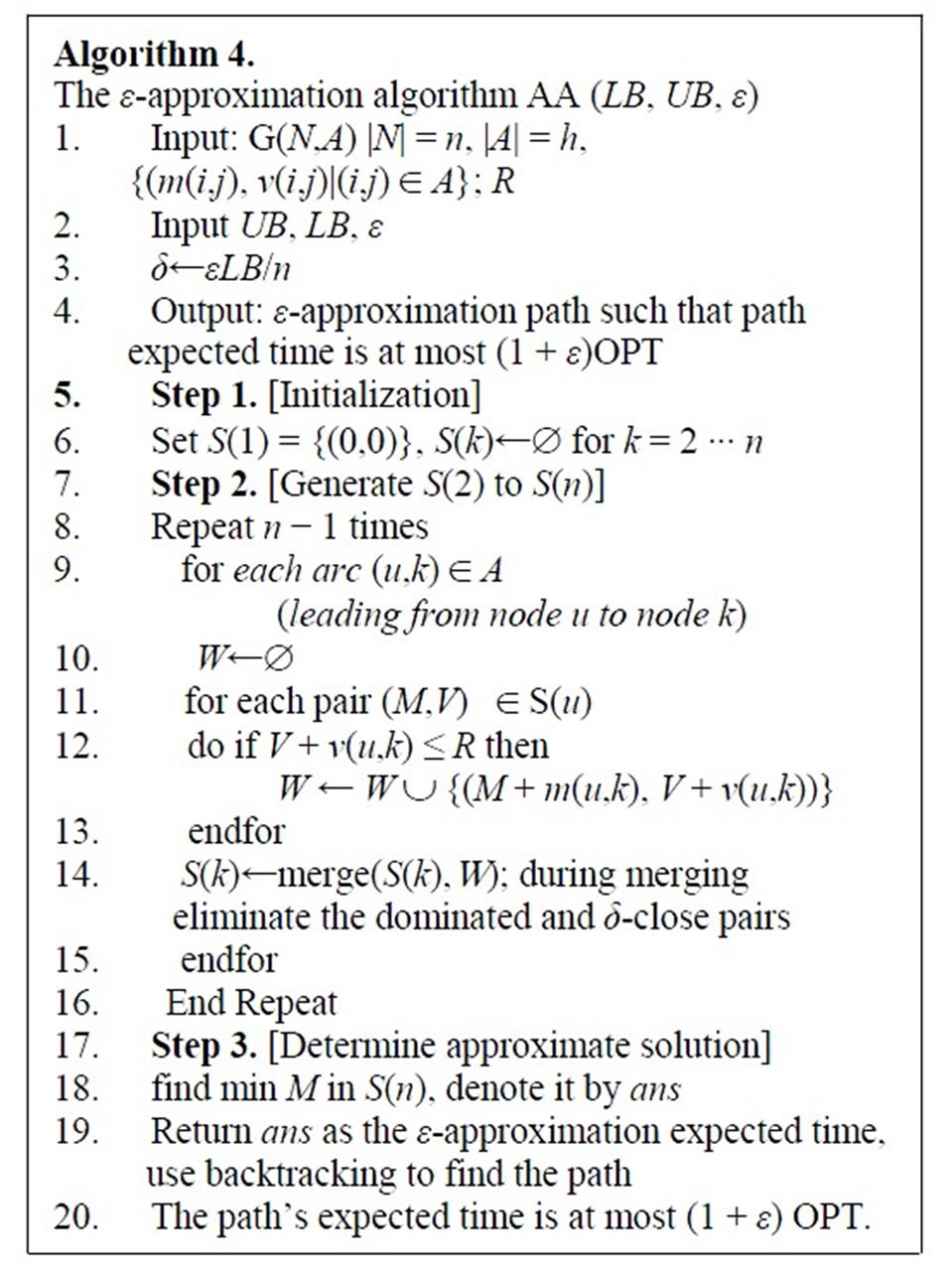
Figure 4. The ε-approximation algorithm AA (LB, UB, ε).
Theorem 1. The complexity of AA (LB, UB, ε) is O(hn2/ε). The complexity of the entire three-stage FPTAS is O(hn2/ε).
Proof: Since the subinterval length is δ = εLB/n, there are O(n(UB/LB)(1/ε)) subintervals in interval [0,UB], and since UB/LB ≤ 2, it comes to O(n/ε) subintervals in interval [LB,UB]. Therefore, there are O(n/ε) representative pairs in any set W, T and S(k). Constructing each W in lines 11 - 13 requires O(n/ε) elementary operations, since W is constructed from a single S(k). Merging the sorted sets W and T, in line 14, as well as discarding all the dominated pairs, is done in linear time (in the number of pairs, which is O(n/ε)). In Step 2 there are O(nh) iterations of lines 11 - 13. Thus, Algorithm 4 has the complexity of O(hn2/ε) in total. Since step C dominates steps A and B of the algorithm, the complexity of the entire approximation algorithm is O(hn2/ε).
6. Example
This section presents a practical numerical example of an application of the model. Figure 5(a) shows a Google Map representation of a region in Tel Aviv. Assume that a car accident has occurred at the point denoted “Accident” on the map, and the nearest ambulance originates from the point denoted “Start”. The destination point for transporting accident victims is the Tel Aviv Sourasky Medical Center, denoted SMC on the map. The ambulance driver needs to choose the route with minimum expected time, satisfying the constraint that the route time variance does not exceed a given threshold R = 4. The corresponding graph with 10 main crossroads and 23 main possible roads is presented in Figure 6. Real-life data are obtained by a statistical survey and presented in Table 1; all the numbers in the table are given in minutes. The last two lines are the average times and corresponding variances. The restricted shortest route found by our algorithm is shown in Figure 5(b). Its total response time is 6.6 with a variance of 3.67, which is less than the allowed value of R = 4. Notice that the shortest unrestricted route in this problem has a total duration of 4.9 minutes,
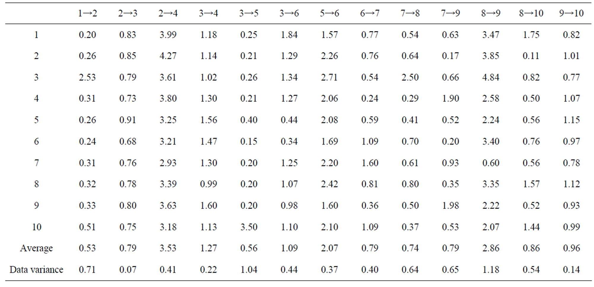
Table 1. Point to point times (in minutes).
 (a)
(a)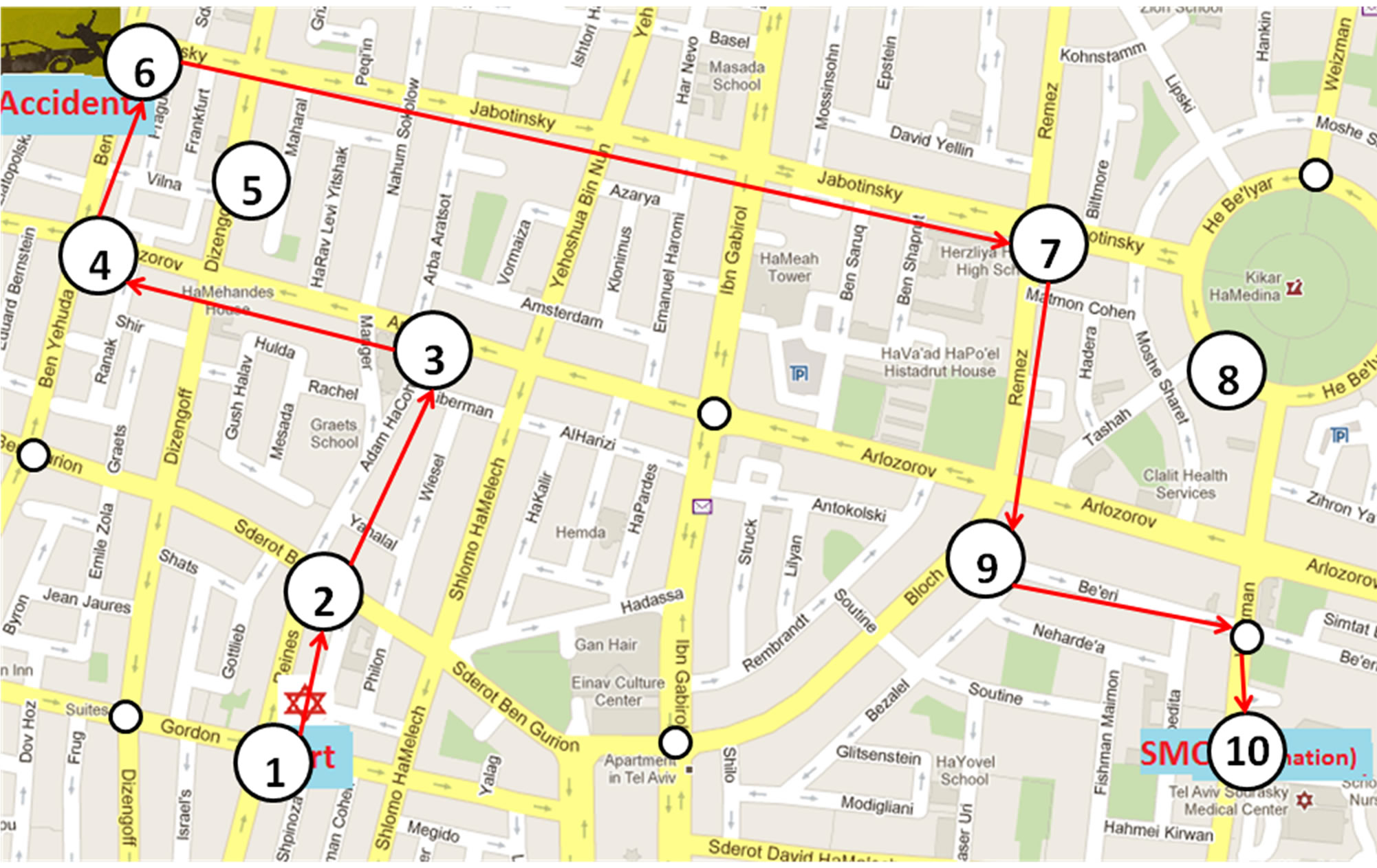 (b)
(b)
Figure 5. (a) Accident area map (Google Maps); (b) A restricted shortest path found.
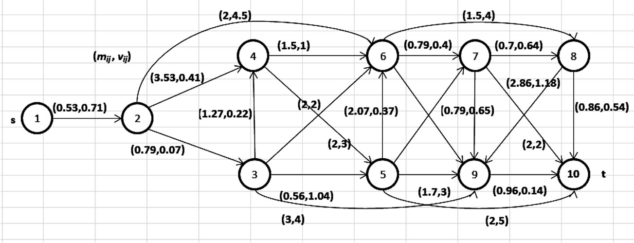
Figure 6. Graph corresponding to main roads.
but its variance is 9.75, which exceeds the given threshold, R = 4. In the worst case, the practical realization of this (random) path duration may be 15 minutes, which is unacceptable in practice.
7. Concluding Remarks
Emergency vehicles are essential for population security. They must respond to emergency situations as quickly as possible and operate under varying conditions. This study improves the state of the art in emergency vehicle routing by introducing stochastic path planning taking the traffic variability into account. The paper’s results demonstrate that stochastic path planning can reduce emergency vehicle travel time in practice. Stochastic path planning shows significant benefits over static path planning. Thus, in situations in which traffic is intensive and highly variable, stochastic path planning can play a significant role in saving lives.
An efficient routing algorithm is an indispensable component of commercial transportation software such as Google Maps [15], GAMS_Transportation Problem Solver [16], and TransCAD [17]. More than that, the constrained routing problem considered in this paper is not only of interest on its own; actually, it arises as a subproblem in many more general optimization problems such as planning and scheduling problems [18], lot-sizing problems [19] and facility location problems [20]. The efficient algorithm for finding the fastest (or cheapest, most profitable, robust, etc.) route usually serves as a subroutine in more general algorithms developed for solving these problems.
This paper proposes an auxiliary dynamic programming approach for developing a fast routing strategy. Since for a large-scale network the complexity of this type of algorithm might be high, a fast approximation algorithm—based on a technique called interval partitioning [9] is introduced. This is the first study to use this approximation technique to solve a problem with uncertain data. To summarize, the mathematical model and algorithms presented in this paper can serve a basis for future real-time emergency vehicle dispatching systems.
They have the following advantages when applied to realtime emergency vehicle routing dispatching:
• The emergency vehicle dispatching model can use real-time traffic information to dynamically compute the shortest paths. The model’s ability to utilize realtime information can improve EVR performance greatly, especially when traffic is dense and there is significant congestion in the road networks.
• The model incorporates a flexible strategy and mathematical optimization using efficient enumeration of numerous routes. This model ensures that the EVR system works efficiently in most real-life situations.
• The system enables responders to handle emergency situations in a timely fashion, i.e., with minimal response times. The proposed algorithm is capable of generating solutions in which travel time variance does not exceed a predetermined threshold; this property is especially important in urban areas with intensive and highly variable traffic. Notice that standard shortest path algorithms do not possess this property. An example of a practical application of the algorithm is given in the previous section.
Future research can expand this work in several directions. First, it would be of interest to develop more realistic model formulations that can handle other types of traffic constraints and additional delay factors encountered in the real world. Along with the typical constraint considered in this paper, according to which the variance of the path travel time cannot exceed a prescribed value, other types of probabilistic constraints are of interest; for instance, future models may pose constraints on the probability that path travel time exceeds a given value. A second potential focus for future work is to design new improved algorithms for solving these models. Furthermore, it would be beneficial both from theoretical and practical points of view to extend the exact and approximation algorithms proposed herein to solve more general lot-sizing and scheduling problems with stochastic parameters. These algorithms could subsequently be compared with the procedures available in existing comercial software systems.
Incorporation of the models and algorithms presented in this paper into a commercial vehicle dispatching system may improve system performance, and assessment of the real-world applicability of these algorithms constitutes another attractive direction for future research.
REFERENCES
- C. Toregas, R. Swain, C. ReVelle and L. Bergman, “The Location of Emergency Service Facilities,” Operations Research, Vol. 19, No. 6, 1971, pp. 1363-1373. doi:10.1287/opre.19.6.1363
- R. Larson, “A Hypercube Queuing Model for Facility Location and Redistricting in Urban Emergency Services,” Computers and Operations Research, Vol. 1, No. 1, 1974, pp. 67-95. doi:10.1016/0305-0548(74)90076-8
- R. Larson, “Approximating the Performance of Urban Emergency Service Systems,” Operations Research, Vol. 23, No. 5, 1975, pp. 845-868. doi:10.1287/opre.23.5.845
- K. Cooke and E. Halsey, “The Shortest Route through a Network with Time-Dependent Internodal Transit Times,” Journal of Mathematical Analysis and Applications, Vol. 14, No. 3, 1966, pp. 493-498. doi:10.1016/0022-247X(66)90009-6
- A. Ziliaskopoulos and H. Mahmassani, “Time Dependent, Shortest-Path Algorithm for Real-Time Intelligent Vehicle Highway System Applications,” Transportation Research Record, Vol. 1408, 1993, pp. 94-100.
- J. Goldberg and L. Paz, “Locating Emergency Vehicle Bases When Service Time Depends on Call Location,” Transportation Science, Vol. 28, No. 4, 1991, pp. 264- 280. doi:10.1287/trsc.25.4.264
- M. Ben-Akiva, E. Cascetta and H. Gunn, “An On-Line Dynamic Traffic Prediction Model for an Inter-Urban Motorway Network,” In: N. H. Gartner and G. Improta, Eds., Urban Traffic Networks: Dynamic Flow Modeling and Control, Springer, Berlin, 1995, pp. 83-122.
- Y. Hadas and A. Ceder, “Shortest Path of Emergency Vehicles under Uncertain Urban Traffic Conditions,” Transportation Research Record, Vol. 1560, No. 1, 1996, pp. 34-39. doi:10.3141/1560-06
- S. Sahni, “Algorithms for Scheduling Independent Tasks,” Journal of the ACM, Vol. 23, No. 1, 1976, pp. 116-127. doi:10.1145/321921.321934
- G. V. Gens and E. V. Levner, “Fast Approximation Algorithms for Job Sequencing with Deadlines,” Discrete Applied Mathematics, Vol. 3, No. 4, 1981, pp. 313-318. doi:10.1016/0166-218X(81)90008-1
- E. Levner, A. Elalouf and T. C. E. Cheng, “An Improved FPTAS for Mobile Agent Routing with Time Constraints,” Journal of Universal Computer Science, Vol. 17, No. 13, 2011, pp. 1854-1862.
- A. Elalouf, E. Levner and T.C.E Cheng, “Efficient Routing of Mobile Agents for Agent-Based Integrated Enterprise Management: A General Acceleration Technique,” Lecture Notes in Business Information Processing, Vol. 88, 2011, pp. 1-20. doi:10.1007/978-3-642-24175-8_1
- T. H. Cormen, C. E. Leiserson, R. L. Rivest and C. Stein, “Introduction to Algorithms,” MIT Press, Cambridge, 2001.
- F. Ergun, R. Sinha and L. Zhang, “An Improved FPTAS for Restricted Shortest Path,” Information Processing Letters, Vol. 83, No. 5, 2002, pp. 287-291. doi:10.1016/S0020-0190(02)00205-3
- R. Gibson and E. Schuyler, “Google Maps Hacks: Tips & Tools for Geographic Searching and Remixing (Hacks),” O’Reilly Media, Inc., 2006.
- A. Brooke, D. Kendrick and A. Meeraus, “GAMS: A User’s Guide,” The Scientific Press, Redwood City, 1998.
- S. Andrews, H. Wang, D. Ni, S. Gao and J. Collura, “Development and Implementation of an Adapted Evacuation Planning Methodology in the Framework of Emergency Management and Disaster Response: A Case Study Using TransCAD,” Journal of Transportation and Security, Vol. 2, No. 4, 2010, pp. 352-368. doi:10.1080/19439962.2010.517743
- M. Pinedo, “Scheduling: Theory, Algorithms, and Systems,” Prentice Hall, Englewood Cliffs, 1995.
- J. R. Evans, “An Efficient Implementation of the WagnerWhitin Algorithm for Dynamic Lot-Sizing,” Journal of Operations Management, Vol. 5, No. 2, 1985, pp. 229-235. doi:10.1016/0272-6963(85)90009-9
- A. D. Klose, “Facility Location Models for Distribution System Design,” European Journal of Operational Research, Vol. 162, No. 1, 2005, pp. 4-29. doi:10.1016/j.ejor.2003.10.031