Intelligent Information Management
Vol.5 No.3(2013), Article ID:31743,9 pages DOI:10.4236/iim.2013.53009
Genetic Algorithm for Concurrent Balancing of Mixed-Model Assembly Lines with Original Task Times of Models
1Department of Mechanical Engineering, Rajalakshmi Engineering College, Anna University, Chennai, India
2Department of Industrial Engineering, College of Engineering, Anna University, Chennai, India
Email: sivasankaranpanneerselvam@yahoo.com, psdeen@gmail.com
Copyright © 2013 Panneerselvam Sivasankaran, Peer Mohamed Shahabudeen. This is an open access article distributed under the Creative Commons Attribution License, which permits unrestricted use, distribution, and reproduction in any medium, provided the original work is properly cited.
Received March 9, 2013; revised April 10, 2013; accepted April 26, 2013
Keywords: Assembly Line Balancing; Cycle Time; Genetic Algorithm; Crossover Operation; Mixed-Model
ABSTRACT
The growing global competition compels manufacturing organizations to engage themselves in all productivity improvement activities. In this direction, the consideration of mixed-model assembly line balancing problem and implementing in industries plays a major role in improving organizational productivity. In this paper, the mixed model assembly line balancing problem with deterministic task times is considered. The authors made an attempt to develop a genetic algorithm for realistic design of the mixed-model assembly line balancing problem. The design is made using the originnal task times of the models, which is a realistic approach. Then, it is compared with the generally perceived design of the mixed-model assembly line balancing problem.
1. Introduction
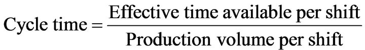
The assembly line balancing problem is basically classified into ALBP 1 and ALBP 2. The ALBP 1 is the type 1 assembly line balancing problem in which the objective is to group the tasks into the minimum number of workstations for a given cycle time, which in turn maximizes the balancing efficiency of the assembly line. The ALBP 2 is the type 2 assembly line balancing problem, in which the tasks are grouped into a given number of workstations such that the cycle time (the maximum of the sum of the task times of the workstations) is minimized. This in turn maximizes the production rate.
The cycle time is computed from the given production volume per shift using the following formula (Panneerselvam 2012).
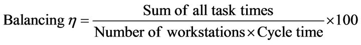
The balancing efficiency of the solution of the line balancing problem is given by the following formula (Panneerselvam, 2012).
In this paper, the ALBP 1 problem with mixed-model is considered. In this problem, there will be many models which are to be produced in batches using the same assembly line. The presence of mixed-model makes the design of the assembly line more complex, in terms of processing times of the tasks and cycle times of the model. The average processing time 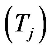 of each task as given by the following formula is normally taken as the representative figure for each task time. If
  for a given i, then the denominator will be decremented by 1.
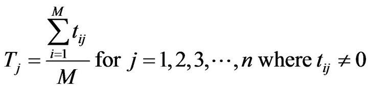
where,
 is the time of the task j in the model i
 is the average time of the task j
 is the number of models
 is the number of tasks In the single model assembly line balancing problem, there will be one cycle time, where as in the mixedmodel assembly line balancing problem, each model will have a cycle time which is normally computed based on the desired production volume per shift of that model. In a problem with two models, if the production volume of Model 1 is 24 assemblies per shift, then the corresponding cycle time is 20 minutes. If the production volume of Model 2 is 48 assemblies per shift, then the corresponding cycle time is 10 minutes. In the case of single model, each cycle time may be considered as such without any modification. In the mixed-model assembly line balanceing problem, the line may be designed for a common cycle time which is computed based on the cycle times of the individual models. If the cycle times of the models are one and the same, then the common cycle time will be equal to the single value; otherwise, the average of the cycle times will be treated as the common cycle time for the problem. Consider Model 1 and Model 2 whose precedence networks are shown in Figures 1 and 2, respectively. The number by the side of each node represents the respective task time. The precedence network for the combined model is shown in Figure 3. In other
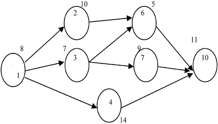
Figure 1. Precedence network of Model 1.
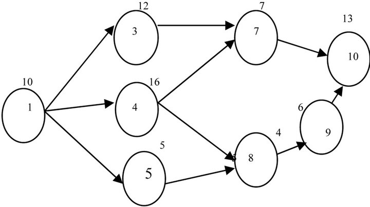
Figure 2. Precedence network of Model 2.
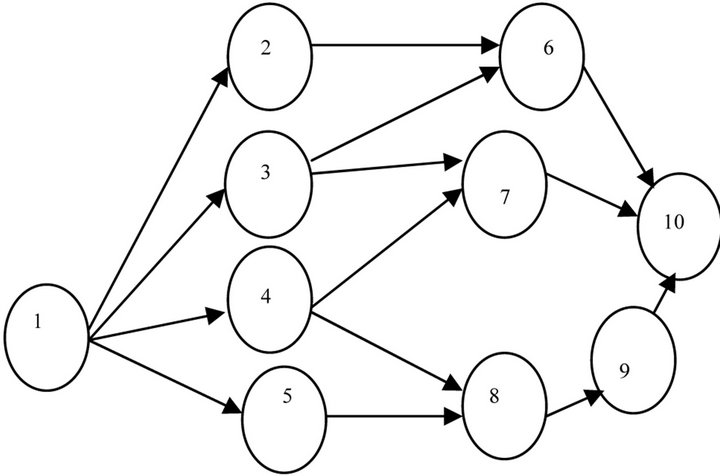
Figure 3. Combined model of Model 1 and Model 2.
works carried out so far in literature, for each task, the authors assumed the average of the times of that task in all the models as the time of that task. If this is followed, after forming the workstations, for some station, there is a possibility that sum of the original times of the tasks which are assigned to that workstation will be more than the cycle time, which will lead to infeasible workstation. Hence, in this paper, the task times of the models are used as such in the design of the assembly line without any modification, which is a major contribution of this research, because it introduces perfection in the solution.
2. Literature Review
This section presents the review of literature of the mixed-model assembly line balancing problem. Gokcen and Erel (1998) have developed a binary integer formulation for of the models. Kim and Kim (2000) have considered the mixed-model assembly line balancing problem. They developed a convolutionary algorithm for balancing and sequencing the assembly line. Matanachai and Yano (2001) have developed a heuristic based on filtered beam search for balancing the mixed-model assembly line to reduce work overload as well as to maintain reasonable workload balance among the stations. Jin and Wu (2002) have considered the mixed-model assembly line balancing problem and developed a heuristic called “variance algorithm” to balance the assembly line. Bukchin and Rabinowitch (2006) have developed a branch and bound based solution approach for the mixed-model assembly line balancing problem to minimize the number of workstations and task duplication costs. Noorul Haq, Zayaprakash and Rengarajan (2006) have developed a hybrid genetic algorithm approach to mixed-model assembly line balancing problem in which the objective is to minimize the number of workstations for a given cycle time. Su and Lu (2007) have considered the mixed-model assembly line balancing problem in which the objective is to design the assembly line to smooth the workload balance within each workstation. They developed a genetic algorithm to find the sequence of models which will minimize the cycle time. They carried out a simulation experiment. Bock (2008) has used distributed search methods for balancing mixed-model assembly lines in the auto industry, in which the objecttive is to minimize the number of workstations. Bai, Zhao and Zhu (2009) have considered mixed-model assembly line balancing problem for which they developed a new hybrid genetic algorithm for finding good solution of the problems.
Ozcan, Cercioglu, Gokcen and Toklu (2010) have considered the balancing and sequencing of parallel mixed assembly lines in which more than one assembly line are balanced together. They have developed a simulated annealing algorithm for this problem to minimize the number of workstations and attain equalization of workstations among workstations. Zhang and Han (2012) have developed an improved differential evolution algorithm for the mixed model assembly line balancing problem applied to car manufacturing industry.
From these literatures, it is observed that the researchers used mathematical models, heuristics, genetic algo rithm, simulated annealing algorithms, etc. to design the assembly line of mixed-models. In all the heuristics as well as meta-heuristics, the combined model of the models is derived and the average time for each task is computed. Then the design of the assembly line is done for a given cycle time common to all the models based on the average task times. Later, the allocation of the tasks to different stations of each model is carried out based on the design of the combined model, which is considered to be unrealistic. Hence, in this paper, an attempt has been made to design the assembly line for the mixed models based on the original timings of the models, which is more realistic. Further, a genetic algorithm is designed to balance the mixed-model assembly line, in which the objective is to minimize the number of stations/ maximize the balancing efficiency.
3. Problem Statement
The problem considered in this paper is the mixed-model assembly line balancing problem. The objective of this research is to group the tasks into a minimum number of workstations without violating precedence constraints for a common cycle time, which is derived, based on the cycle times of the models. Generally, the common cycle time is the average of the cycle times of the models. In this paper, a genetic algorithm is designed for the mixedmodel assembly line balancing problem, in which the original times of the tasks are used while concurrently designing the workstations of the models.
4. Genetic Algorithm
This section presents a genetic algorithm for designing mixed-model assembly line balancing problem. It uses cyclic crossover to obtain offspring.
Consider the combined precedence network of assembling the Model 1 and Model 2, which has ten tasks, as shown in Figure 3. Each chromosome in the original population is generated by randomly assigning the tasks to different gene positions in the chromosome. Two sample chromosomes for the tasks in Figure 3 are shown in Tables 1 and 2.
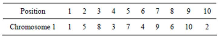
Table 1. Chromosome 1.
The cyclic crossover method presented by Senthilkumar and Shahabudeen (2006) gives two offspring from the chromosome 1 and the chromosome 2 as shown in Table 3.
4.1. Construction of Ordered Vector
The genes of each chromosome are to be ordered (rearranged) such that the serial assignment of the genes from the ordered vector to workstations does not violate the precedence constraints as shown in the Figure 1 as well as in the Figure 2. The steps of constructing ordered vector for a given chromosome/offspring are presented in Annexure 1.
The application of the steps to the chromosome 1 shown in Table 1 gives an ordered vector as shown in Table 4.
4.2. Evaluation of Fitness Function of Chromosome
The fitness function of the chromosome 1, namely balancing efficiency is obtained by assigning the tasks serially from left to right from its ordered vector 1-5-3-4-8- 7-9-2-6-10 into workstations for a given cycle time of 20 units as shown in Table 5. It is assumed that the cycle time of the model 1 as well as that of the model 2 as 20 minutes. Hence, the cycle time of the combined model is also 20 minutes, which is the average of the cycle times of both the models.
While assigning a task into a workstation, that task pertaining to all the models should be assigned to the same workstation. If a task is available in only one model then that can be independently assigned to the current workstation. The allocations of the tasks to different workstations of both the models are pictorially shown in Figure 4.
4.3. Steps of GA Based Heuristic with Cyclic Crossover Method
The steps of GA based heuristic with cyclic crossover
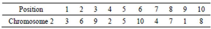
Table 2. Chromosome 2.
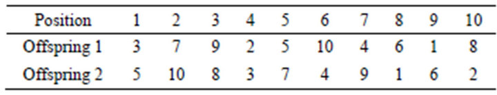
Table 3. Offspring of chromosomes 1 and 2.
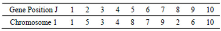
Table 4. Ordered vector of chromosome 1.
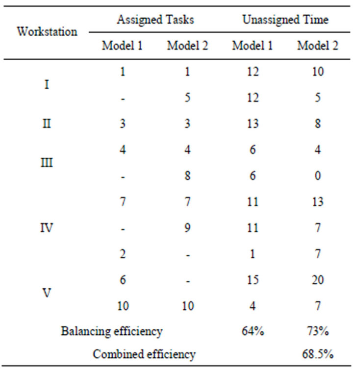
Table 5. Solution for the ordered vector 1-5-3-4-8-7-9-2-6- 10.
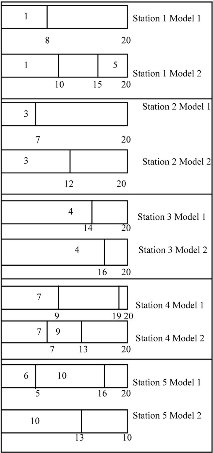
Figure 4. Assignment of tasks to workstations.
method to group the tasks of the mixed-model assembly line balancing problem into a minimum number of workstations are presented in Figure 5. Here, the balancing efficiencies of the individual models and the balancing efficiency of the combined model are maximized.
5. Comparison of Proposed Ga Results with Conventional Ga Results
This section gives the comparison of the results of the proposed GA algorithm with that of the generally perceived genetic algorithm using the example given in Section 1. In the genetic algorithm, the number of iteration is 20. The size of the population and that of the sub-popu-
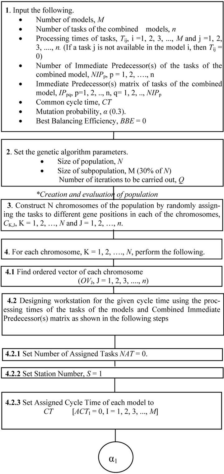

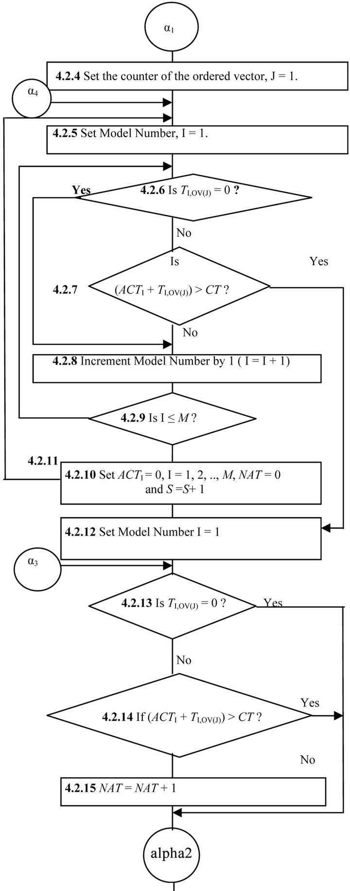
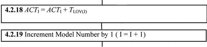
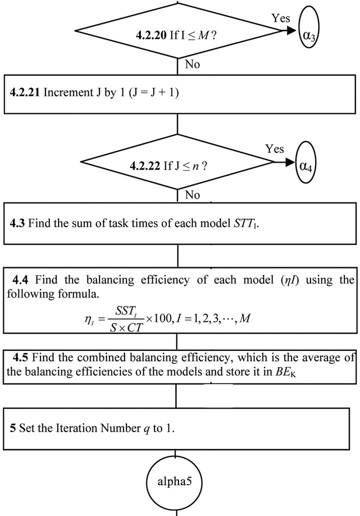
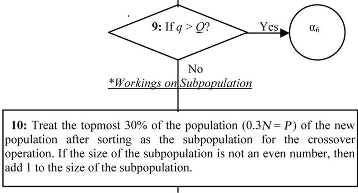
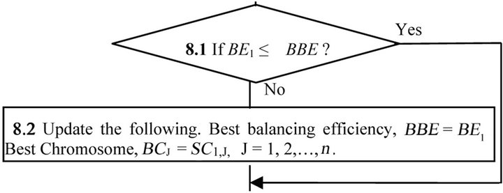


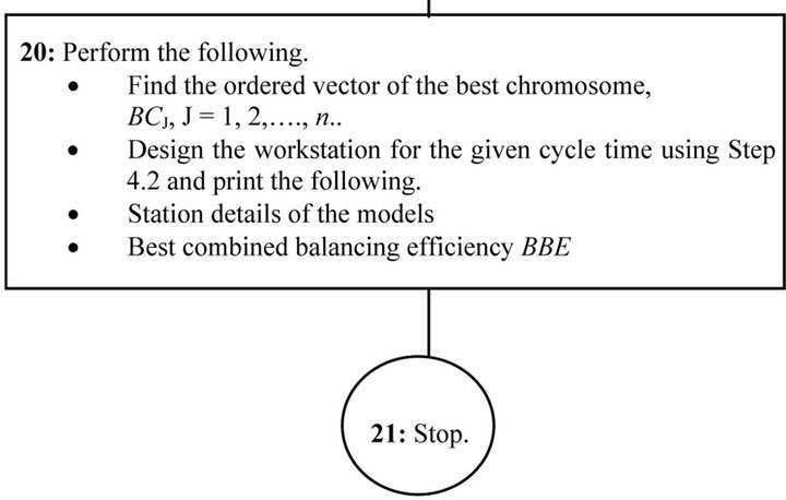
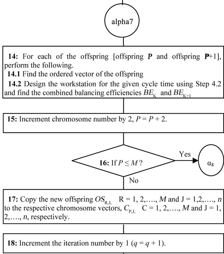
Figure 5. Steps of GA based heuristic with cyclic crossover method.
lation are 50 and 20, respectively.
5.1. Results of Proposed Genetic Algorithm
The application of the proposed genetic algorithm to the example problem shown in Section 2 gives the best chromosome and the corresponding ordered vector as shown in Table 6. The details of the stations of the Model 1 and Model 2 are shown Table 7. The allocations of the task to different workstations of both models are shown in Figure 6.
5.2. Results of Generally Perceived Genetic Algorithm
Generally all the researchers use the combined precedence network, average processing times of the tasks to design the assembly line for the common cycle time of the combined model. The average time of the tasks are shown in Table 8. It should be noted that the average time of a task is computed by dividing the sum of the task times in all the models of that task where it is present, by the number of models in which that task is present. But, in past researches, for a given task, the average task time is obtained by dividing the sum of that task times in
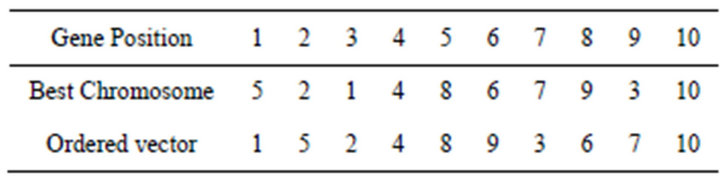
Table 6. Best chromosome and corresponding ordered vector.
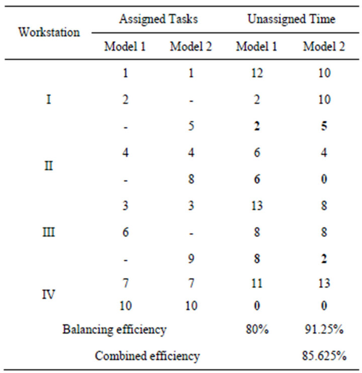
Table 7. Solution using the proposed genetic algorithm with individual task times of the models.
all the models by the number of models, which is a wrong approach.
The application of the generally perceived genetic algorithm with cyclic crossover gives the best chromosome and the corresponding ordered vector as shown in Table 9.
For the ordered vector shown in Table 9, the assemblyline balancing (ALB) results using the generally perceived genetic algorithm with average task times are already shown in Table 5. The allocations of the tasks to different workstations of both models for this solution are already pictorially shown in Figure 5.
The comparison of balancing efficiencies of the generally perceived GA (GP-GA) and proposed GA (P-GA), which is shown in Tables 5 and 7, respectively is shown
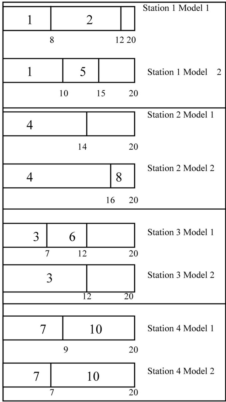
Figure 6. Assignment of tasks to workstations.

Table 8. Average task times of the combined model.
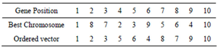
Table 9. Best chromosome and ordered vector using generally perceived genetic algorithm.
in Figure 7. From the Figure 7, it is clear that the balancing efficiencies of the individual models using P-GA are better than that that of the individual models using GP-GA. The comparison of combined balancing efficiencies of GP-GA and P-GA is shown in Figure 8. From the Figure 8, it is seen that the proposed GA performs better than the generally perceived GA, in terms of combined balancing efficiency.
6. Conclusions
The mixed-model assembly line balancing gives a greater challenge to the designers in industries in terms of dealing with different models. The researchers use the average times of the tasks of the models as the timings of the tasks of the combined model while designing the line. But, this is an approximation method of dealing with the data. Hence, in this paper, the design of the assembly line of the models is done concurrently for all the models using their original task times. Such an attempt gives a realistic design of the mixed-model assembly line.
A genetic algorithm is designed to balance the assembly lines of the models of the mixed-model assembly line balancing problem. In this algorithm, a cyclic crossover
GP-GA P-GA
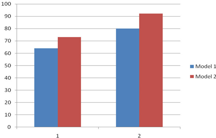
Figure 7. Comparison of balancing efficiencies of models using GP_GA and P-GA.
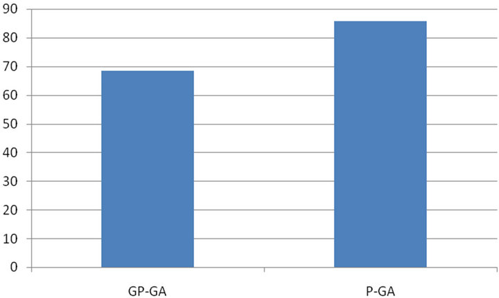
Figure 8. Comparison of combined balancing efficiencies of GP-GA and P-GA.
method is used to perform crossover operation between chromosomes. The superiority of this approach is demonstrated using a numerical example. The proposed genetic algorithm with cyclic crossover and with individual task times of the models is a unique contribution to literature, because in the past all the researchers used average times of the tasks of the combined model to form the stations which is an approximate method of balancing.
7. Acknowledgements
The authors thank the anonymous referees for their constructive suggestions, which have improved the paper.
REFERENCES
- Y. Bai, H. Zhao and L. Zhu, “Mixed-Model Assembly Line Balancing Using the Hybrid Genetic Algorithm,” International Conference on Measuring Technology and Mechatronics Automation, Zhangjiajie, 11-12 April 2009, pp. 242-245.
- S. Bock, “Using Distributed Search Methods for Balancing Mixed-Model Assembly Lines in the Automotive Industry,” OR Spectrum, Vol. 30, No. 3, 2008, pp. 551-578. doi:10.1007/s00291-006-0069-9
- Y. Bukchin and I. Rabinowitch, “A Branch-and-Bound Based Solution Approach for the Mixed-Model Assembly Line-Balancing Problem for Minimizing Stations and Task Duplication Costs,” European Journal of Operational Research, 174, No. 1, 2006, pp. 492-508. doi:10.1016/j.ejor.2005.01.055
- H. Gokcen and E. Erel, “Binary Integer Formulation for Mixed-Model Assembly Line Balancing Problem,” Computers & Industrial Engineering, Vol. 34, No. 2, 1998, pp. 451-461. doi:10.1016/S0360-8352(97)00142-3
- M.-Z. Jin and S. D. Wu, “A New Heuristic Method for Mixed-Model Assembly Line Balancing Problem,” Computers & Industrial Engineering, Vol. 44, No. 1, 2002, pp. 159-169. doi:10.1016/S0360-8352(02)00190-0
- Y. K. Kim and J. Y. Kim, “A Co-Evolutionary Algorithm for Balancing and Sequencing in Mixed-Model Assembly Lines,” Applied Intelligence, Vol. 13, No. 3, 2000, pp. 247-258. doi:10.1023/A:1026568011013
- S. Matanachai and C. A. Yano, “Balancing Mixed-Model Assembly Lines to Reduce Work Overload,” IIE Transactions, Vol. 33, No. 1, 2001, pp. 29-42. doi:10.1080/07408170108936804
- A. N. Ha, J. Jayaprakash and K. Rengarajan, “A Hybrid Genetic Algorithm Approach to Mixed-Model Assembly Line Balancing,” International Journal of Advanced Manufacturing Technology, Vol. 28, No. 3-4, 2006, pp. 337-341. doi:10.1007/s00170-004-2373-3
- U. Ozcan, H. Cercioglu, H. Gokcen and B. Toklu, “Balancing and Sequencing of Parallel Mixed-Model Assembly Lines,” International Journal of Production Research, Vol. 48, No. 17, 2010, pp. 5089-5113. doi:10.1080/00207540903055735
- R. Panneerselvam, “Production and Operations Management,” 3rd Edition, PHI Learning Private Limited, New Delhi, 2012.
- P. Senthilkumar and P. Shahabudeen, “GA Based Heuristic for the Open Shop Scheduling Problem,” International Journal of Advanced Manufacturing Technology, Vol. 30, No. 3-4, 2006, pp. 297-301. doi:10.1007/s00170-005-0057-2
- P. Su and Y. Lu, “Combining Genetic Algorithm and Simulation for the Mixed-Model Assembly Line Balancing Problem,” 3rd International Conference on Natural Computation (ICNC 2007), Vol. 4, Haikou, 24-27 August 2007, pp. 314-318.
- X. M. Zhang and X. C. Han, “The Balance Problem Solving of the Car Mixed-Model Assembly Line Based on Hybrid Differential Evolution Algorithm,” Applied Mechanics and Materials, Vol. 220-223, 2012, pp. 178- 183. doi:10.4028/www.scientific.net/AMM.220-223.178
Annexure 1. Steps of Construction of Ordered Vector
The steps of constructing ordered vector are presented in this appendix.
Step 1: Input the chromosome.
Ÿ Let the chromosome I be as shown in Table A1 along with the values for the STATUS row as zero. If the value of the STATUS for a gene (task) is zero, then it signifies that it is not assigned to any workstation; otherwise, it signifies that it is assigned to some workstation.
Ÿ Form the immediate predecessor(s) matrix of the tasks of the combined model as shown in Table A2. The maximum of the number of immediate predecessors in Figure 3 is 3.
ŸNumber of tasks (genes of the chromosome), N
ŸInitialize gene position of the ordered vector, 
Step 2: Set the gene position of the chromosome, 
Step 3: If the STATUS of the gene J of the chromosome I is equal to 1, then go to Step 9; else, go to Step 4.
Step 4: If all the immediate predecessors values in the Table 9 with respect two the task at the gene position J of the chromosome I are zero, then go to Step 5; otherwise, go to Step 9.
Step 5: Assign the task at the gene position J of the chromosome I to the gene position K of the ordered vector. 
Step 6: Set the status of the gene position J of the chromosome I to 1. 
Step 7: Change the value of  in immediate predecessor matrix to zero, wherever it appears in it.
Step 8: Increment the gene position (K) of the ordered vector by 1 and go to Step 2.
Step 9: Increment the gene position (J) of the chromosome by 1.
Step 10: If , then go to Step 3; else go to Step 11.
Step 11: Stop.
Table A1. Chromosome I.
| Gene Position J | 1 | 2 | 3 | 4 | 5 | 6 | 7 | 8 | 9 | 10 |
| STATUS | 0 | 0 | 0 | 0 | 0 | 0 | 0 | 0 | 0 | 0 |
| Chromosome 1 | 1 | 5 | 8 | 3 | 7 | 4 | 9 | 6 | 10 | 2 |
Table A2. Immediate predecessor(s) matrix [IPpq].
| Task (p) | Immediate Predecessor(s) (q) | ||
| 1 | Nil | ||
| 2 | 1 | ||
| 3 | 1 | ||
| 4 | 1 | ||
| 5 | 1 | ||
| 6 | 2 | 3 | |
| 7 | 3 | 4 | |
| 8 | 4 | 5 | |
| 9 | 8 | ||
| 10 | 6 | 7 | 9 |