iBusiness
Vol. 4 No. 4 (2012) , Article ID: 25646 , 9 pages DOI:10.4236/ib.2012.44039
Performance Evaluation Study on Supply Chain for Short-Life-Circle Products—Illustrated by the Case of LCD TV
![]()
1School of Business, Central South University, Changsha, China; 2School of Business, Hunan University of Technology, Zhuzhou, China; 3School of Finance , Hunan University of Technology, Zhuzhou, China.
Email: shellyzx2405@163.com
Received May 24th, 2012; revised June 24th, 2012; accepted July 24th, 2012
Keywords: Short-Life-Circle; Supply Chain for LCD TV; Bass Model; Simulation Analysis
ABSTRACT
According to the characteristics of short-life-cycle products analyzed, we adopted Bass-model method to forecast the demand for products and proposed a research framework based on simulation. Meanwhile, study the influence degree of every experimental variable (including demand form and each uncertainty, etc.) on supply chain for LCD TV aiming at typical supply chain for LCD TV and adopt the performance indexes such as total profit, total finished goods quantity, fill rate, and flow time to the relevant example analysis and validation.
1. Introduction
The rapid step of new product introduction has led to the continuously shortening of product life cycle in many industries. That lots of product life cycles have been shortened by several months or two years at most. The popular industries (such as toy and dress) and high-tech industries (for example: computer, LCD screen, LCD TV and consumptive electronic product) has been widely distributed. The typical demand form of short-life-cycle product experiences rapid growth, maturity and recession of the three stages, most of which show s curves. According to related information of manufacturers, LCD TV is a typical short-life-cycle product for the updating time of its new product is about two years, and the cumulate demand on single type product (42 inches of LCD TV) presents also s curve. The demand forecast methods such as traditional moving average and exponential smoothing are only suitable for the condition that the demand trend and season tend to be table with time; complicated BoxJenkins method is mainly applied to the condition that there is lots of historical information of demand. So we can use Bass model to forecast product demand directing to the demand features of short-life-cycle product.
By proposing a stimulant basic research framework, This research aimed to discuss the influence degree of each experimental variable on supply chain in LCD TV (including demand form, order grace level, every uncertainty, etc.), and evaluate the manifestations of every demand form on the basis of different performance indexes in different environment. We used the performance indexes such as total profit, quantity of total finished goods; fill rate and flow time to demonstrate the proposed research framework.
2. Literature Review
Among the abroad related researches, Pasternack (1985) studied the buy-back mechanism of supply chain for short-life-cycle products. The supply chain model, constructed by Pasternack, consisted of the single manufacturer and distributor. In this model, the manufacturer committed to buy back the rest products unsold by distributor with below the wholesale price after the end of season to achieve the coordination of production and marketing by effective incentive wholesale price and buy-back price [1]. Kurawarwala and Matsuo (1998) predicted the demand for short-life-cycle products by using the linear growth model, index growth model and seasonal trend growth model. The personal computer with 38 months of life cycle was taken as example, and the demand was based on the historical materials of past products. The study indicated that seasonal trend growth model was the best and the linear growth model was the worst [2]. Higuchi and Troutt (2004), taking Tamagothchi (a kind of virtual pet toy) as example, investigated the supply chain for short-life-cycle products and, forecasted the demand for short-life-cycle products by using the dynamic simulation method based on situation and Logistics curve (S curve) adopted by distributors [3].
In domestic researches, Xu Xianhao (2007) indicated the predicting method on demand for short-life-cycle products based on diffusion theory. He summarized the present researches on demanding prediction of short-lifecycle products in domestic and abroad researches, analyzed deeply the related features of demand on short-lifecycle products, and then studied the general approach of demanding prediction of short-life-cycle products in the basis of the features [4]. Ding Lijun, Liu Bin, et al. (2004) studied how to coordinate the supply chains of twice producing and ordering mode for the seasonal products with long production lead time and short sale season in the two-stage supply chain model composed of one manufacturer and one distributor. And according to the characteristics of dull sale subsidy contract and return contract, he established effective contract model and verified the influences of the model on the manufacturer’s producing and ordering activities in supply chain through specific simulation examples [5,6]. T. P. Zhang, S. J. Li, et al. proposed and established the performance evaluation index system based on the overall effectiveness of supply chain, and divided the performance index of supply chain into three levels: strategy performance index, tactic performance index and operation performance index. At the same time, each specific index was defined and given the responding index calculation or qualitative judging [7,8].
To summarize the above literatures, the demanding morphology of short-life-cycle products has its uniqueness, mostly showing the S curve. So it needs to be distinguished with the general life-cycle products. Although there are many researches on short-life-cycle products presently and a few of researches on the supply chain for short-life-cycle products, the studies on performance evaluation of supply chain under the characteristics of shortlife-cycle are still limited, especially there are short of the studies on demand morphology and various uncertainties, which provides a simulation study space for this paper.
3. Research Methods and Architecture
3.1. Research Framework
We put forward a research architecture based on simulation as shown in Figure 1: it is a simulation program in the central part of which the input terminal includes supply chain for LCD TV, system parameters and experimental variables; and the output terminal is performance index. According to the research framework, we discuss the influence degree of each experimental variable (embracing demand form, order allowance level, various uncertainties, etc.) on supply chain for LCD TV based on
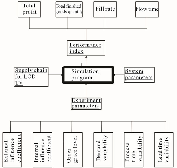
Figure 1. The operation of manufacture.
every performance index and evaluate the manifestation of each demand form in terms of different performances indexes.
3.2. Supply Chain for LCD TV
A typical supply chain for LCD TV is studied in this research, and a number of suppliers of raw materials, one manufacturer and many customers are involved in the members of supply chain. The supply chain belongs to the order production (MTO) which means that the manufacturer prepare materials/parts in the light of customer’s order, and then send the finished goods to customer in committal time after the manufacturing process of LCD TV. The manufacturer adopts the (S, Q) of inventory policy that is when the inventory of one certain material/ part is lower than the reorder point (S), the manufacturer will order a specific volume (Q) of material/part to other suppliers [9]. The operation flow is described as Figure 1.
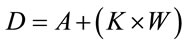
Firstly the orders should be integrated on the basis of customer requirements in the day unit, so the orders enter pending order area to wait, then the production operation begins, lastly manufacturer transforms the finished goods to customer in committal time. Since each order should be set due date firstly, we use TWK (total work content) method to set it. This method is used widely for the best delay related performance can be got with it. The method is based on the following formula:
 (1)
(1)
In this formula:
D represents order due date;
A represents order arrival time;
K represents allowance level, constant, the bigger the K is, the more the due date is delayed;
W represents content of operation, refers to the comprehensiveness of average treatment time when the order is at each operation.
The reorder lead time of material/part, treatment time of each operation and transportation time of finished goods are all uncertain in this article. Additionally, there is lack of direct historical data to any new product in the short life cycle, but there usually exist the sales data about the complete life cycle of previous generation or similar products which have very high value on forecasting the demand on future products. However most of companies regard the complete sales data of single type product especially the previous generation as the commercial confidential information, thus we hypothesize in the research that the sales data about complete life cycle of previous generation products can be used to establish suitable Bass diffusion model which is applied to forecasting the demand on new product.
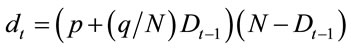
According to the hypothesis of Bass diffusion model, the potential users of new product are divided into two groups: one group is influenced by mass media and the other one is influenced only by public praise; the former is called “innovation adopter” and the latter is called “imitator” [10]. Bass diffusion model can be described as the following formula:
 (2)
(2)
In this formula:
dt represents the demand on time t;
Dt−1 represents the cumulative demand by the time t − 1;
p represents external influence coefficient;
q represents internal influence (imitation) coefficient;
N represents the potential total demand of market (namely the maximum possible value of Dt).
3.3. Experimental Variables
We focus on demand form and (the combination of each Bass diffusion model parameter) and various uncertainties to understand whether the different experimental variables have significant impact on the supply chain for LCD TV and consider every variable that may influence the system. The followings are the experimental variables applied in this research, respectively:
1) External influence coefficient-Bass diffusion model parameter (p), stands for innovation or degree of external influence;
2) Internal influence coefficient-Bass diffusion model parameter (q), stands for imitation or degree of internal influence;
3) Order grace level-estimate the due date of order by TWK method, need to set grace level firstly;
4) Demand variability (DDV)-variability coefficient, the ratio between standard deviation and average, stands for demand variability degree in this research;
5) Process time variability (LTV);
6) Lead time variability (LTV).
3.4. Performance Index
We introduce four universal performance indexes in researches on general supply chain, as following:
1) Total profit (TP) represents the total profit of system during the effective data collection; total profit is the difference between total income and total cost; and the total cost is the product of total completed number that send to customer and unit price of finished product.
The monomial cost accountings that contained in total cost are: purchasing cost of material/part (including transportation cost), holding cost of material/part, treatment cost in LCD TV production, transportation cost of finished goods, punishment cost for late delivery of order, and so on.
2) Quantity of total finished goods-refers to the total finished number that complete the assembly of products and deliver them to client during the effective data collection.
3) Fill rate (FR) refers to the ratio between the orders delivered to clients in manufacturer’s promised time and the total orders.
4) Flow time (FT) represents the time from receiving orders to transforming the finished goods to clients, including the waiting time before order off-line, time on off line and time that costs on transforming finished goods to clients.
3.5. Research Tools
The simulation software Extend Suite v6 is regarded as research tool to establish simulation model in this study.
4. Example Analysis
4.1. Illustration Explanation
The example indicates that this study is based on an actual “supply chain for LCD TV” which belongs to threestage supply chain, involving a number of suppliers of raw materials, one manufacturer and many clients.
4.2. System Parameters Setting
We have to set complete system parameters to define the operating environment of the whole supply chain for LCD TV, as shown in Table 1. These data are provided by each case company. The materials of processing time of job, delivery time of finished product and lead time of material/part are collected actually. The results of analysis on them are distributed with Lognormal. Additionally,
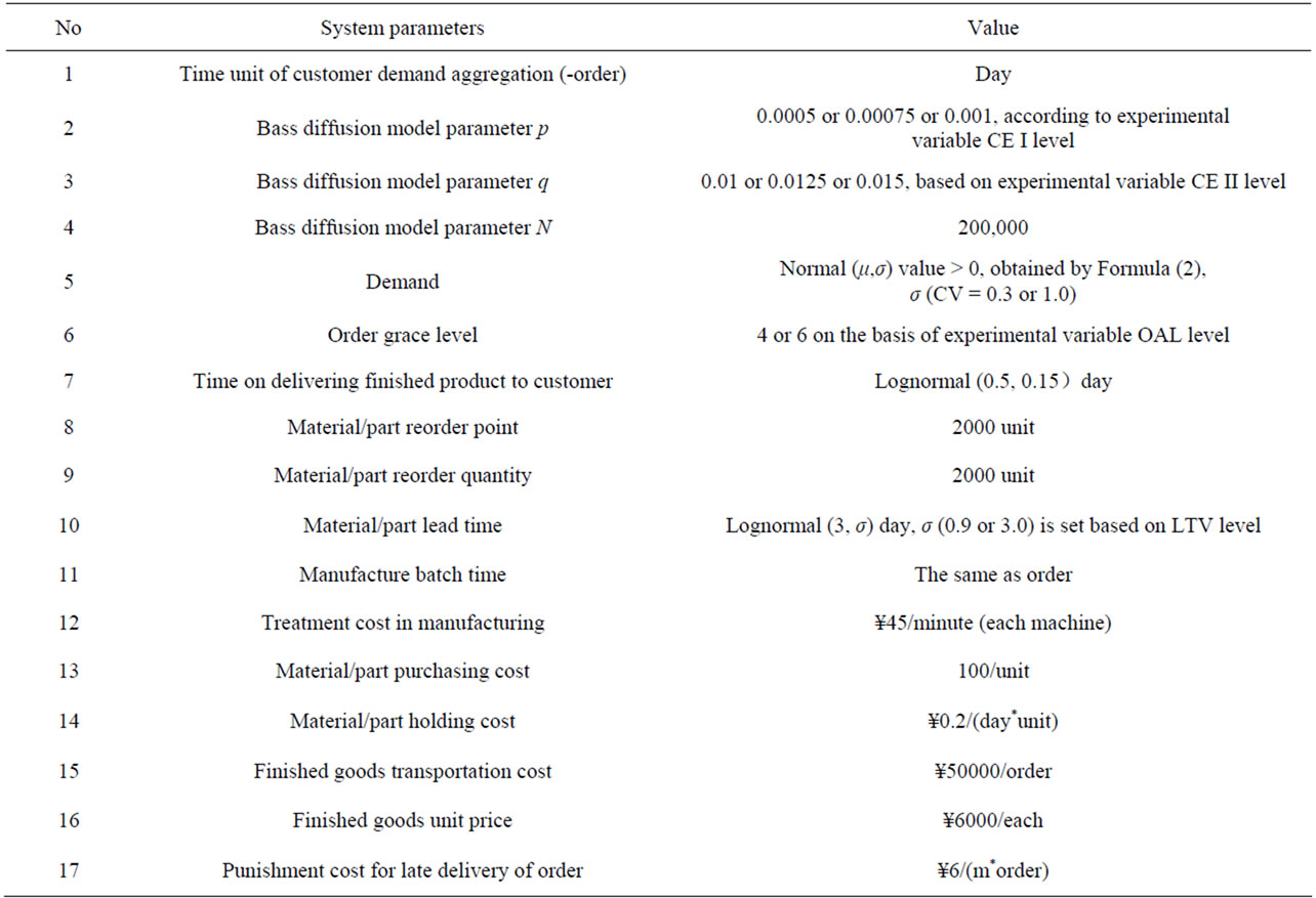
Table 1. System parameters setting.
it should be noted that the values of some system parameters are decided in the basis of experimental variables.
4.3. Experimental Parameters Setting
Each experimental parameter is referring to two standards in this example, as shown in Table 2. The principle of selecting standard is that the led performance indexes should show significant difference according to different standards. Besides consulting the experts of each case company, some standards are measured by a series of tests. And the level 1 of external influence coefficient and internal influence coefficient represents the low degree of influence coefficients; the level 2 is on behalf of the high degree of influence coefficient; On the uncertainties, CV = 0.3 represents the low-degree variability, and CV = 1.0 is on behalf of high-degree variability.
5. Simulation Results and Analysis
Tables 3 and 4 represent the manifestations of supply chain for LCD TV in any experiment and performance index when CEI is equal to level1 (low-degree CEI) and level 2 (high-degree CEI), respectively. The data of each column in the table are the averages and standard deviations of results which are performed ten times. Besides, according to the simulation results, we analyze the variation amount to find out which factors can influence significantly the performance of supply chain for LCD TV, and the outcome is shown as Table 5 (directing against every performance index). Since the interaction of two factor and above on system performance is little, this research emphasizes on the discussion on the single factor.
5.1. Total Profit
The p values of CEI and CEII are more less than 0.05 from the analysis on the variation amount of total profit, which shows they have remarkable impact on total profit, and so does the order grace level; and the three variables of uncertainty (demand variability, processing time variability and Lead time variability) all influence the total profit remarkably.
In the part of external influence coefficient, the results of simulation experiment displays that the total profit is higher under the low-degree external influence coefficient (CEI = L1) than the high-degree external influence coefficient (CEI = L2). The reason is that demand curve is flat, and the highest point of curve is low relatively on
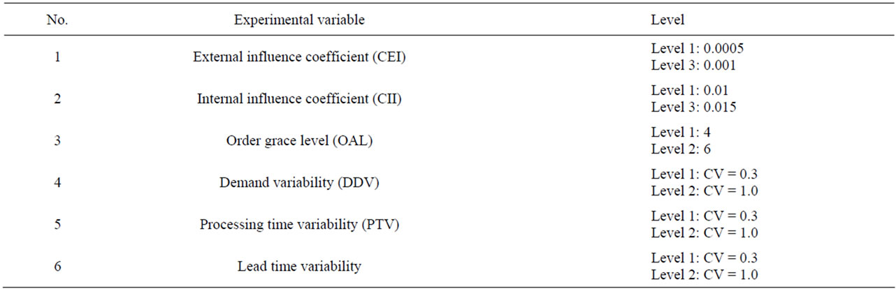
Table 2. Experimental variable level setting.
the condition of low-degree external influence coefficient and, the simulation data also displays that the purchasing cost, holding cost and punishment cost for late delivery of order are all low, so the total profit is high.
In the part of order grace level (OAL), the total profit under the condition of high order grace level (OAL = L2) is higher than low grace level (OAL = L1) on the basis of the outcome of simulation experiment. Because the short order delivery causes easily the late delivery of orders on the condition of low order grace level, which increases the punishment cost, consequently, the total profit is low.
On processing time variability (PTV), the results of simulation experiment exhibit that the total profit is higher on low variability (PTV = L1) than high variability (PTV = L2). On high variability, the processing time is not steady, so when it is elongated, the orders waiting in temporary storage areas of every operation and the numbers of total finished goods are both influenced, which leads to high treatment cost, high punishment cost and low income, consequently the total profit is low.
Remark:
1) CEI represents external influence coefficient, CII represents internal influence coefficient, OAL represents order grace level, DDV represents demand variability, PTV represents treatment time variability, LTV represents lead time variability of raw material/part;
2) L1 represents Level 1, L2 represents Level 2;
3) Unit of each performance index: total profit-kg, number of total finished goods-each, flow time-day.
In the part of lead time (LTV) of material/part, the results of simulation experiment exhibit that the total profit is higher in the situation of low variability (PTV = L1) than high variability (PTV = L2). In the situation of high variability, the lead time of material/part is not steady, so when it is elongated, the production is delayed for lack of materials/parts, then the orders waiting in temporary storage areas of every operation and the quantity of finished goods are both influenced, which leads to high treatment cost, high punishment cost and low incomethus the total profit is low.
5.2. Quantity of Total Finished Goods (QF)
The p values of CEI and CEII both are more than 0.05 from the analysis on the variation amount of total quantity of finished goods, which shows there has no remarkable impact on total profit, and so does the order grace level; there are two variables (demand variability and processing time variability) among uncertain variables have significant impact on total quantity of finished goods. In terms of demand variability, the results of simulation experiment seen from Tables 3 and 4. The results show that there are more finished goods on the condition of high variability (DDV = L2) than low variability (DDV = L1). The reason is that the large change of demand causes the high quantity of finished goods.
In the part of processing time variability (PTV), there is higher quantity of finished goods on condition of low variability (PTV = L1) than high variability (PTV = L2). Because the processing time is not steady in the situation of high variability, and when the processing time is elongated, the orders waiting in temporary storage areas of every operation are influenced, therefore the total quantity of finished goods is low.
Remark:
1) CEI represents external influence coefficient, CII represents internal influence coefficient, OAL represents order grace level, DDV represents demand variability, PTV represents treatment time variability, LTV represents lead time variability of raw material/part;
2) L1 represents Level 1, L2 represents Level 2;
3) Unit of each performance index: total profit-kg, number of total finished goods-each, flow time-day.
5.3. Fill Rate
Seen from the analysis on variance of fill rate in Table 5, the p values of external influence coefficient (CEI) and internal influence coefficient (CII) are more less than

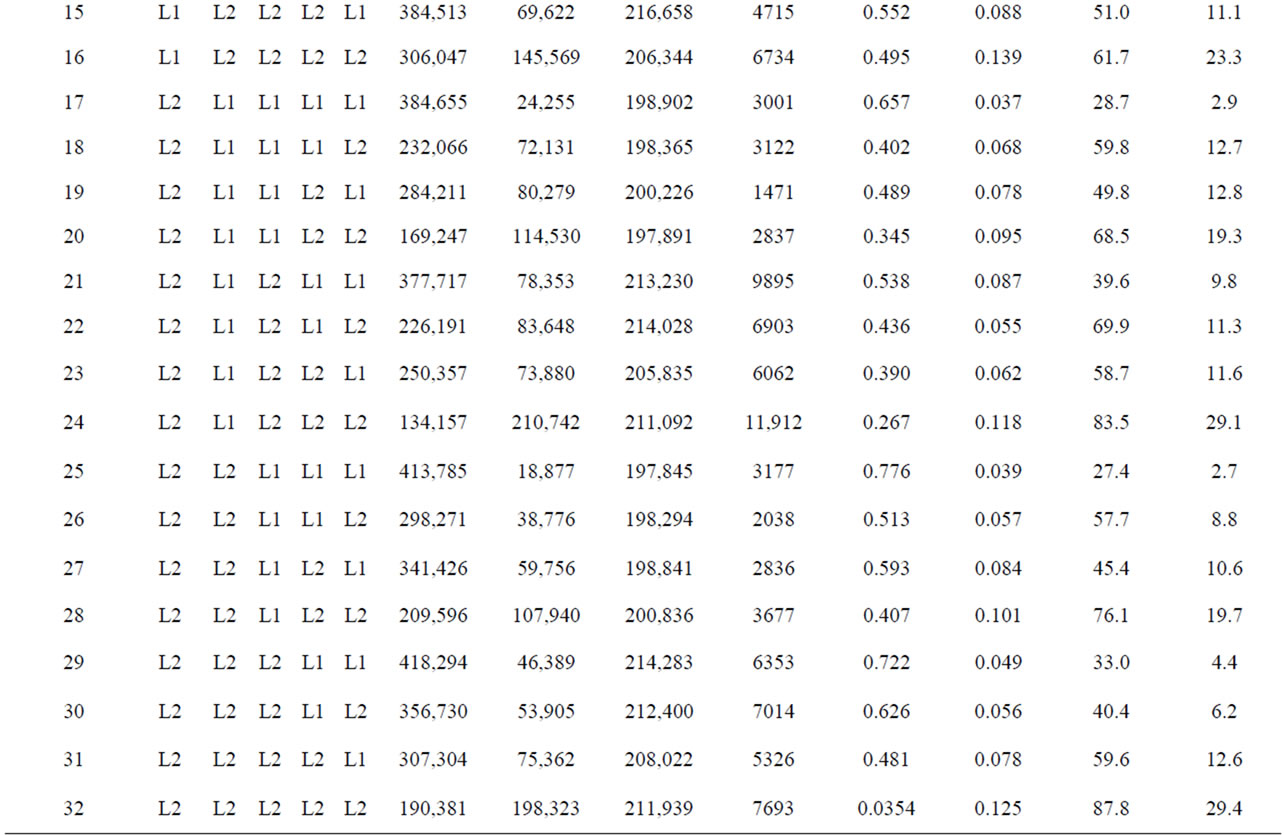
Table 3. Simulation results-ECI = L1 (low-degree external influence coefficient).


Table 4. Simulation results-ECI = L2 (high-degree external influence coefficient).
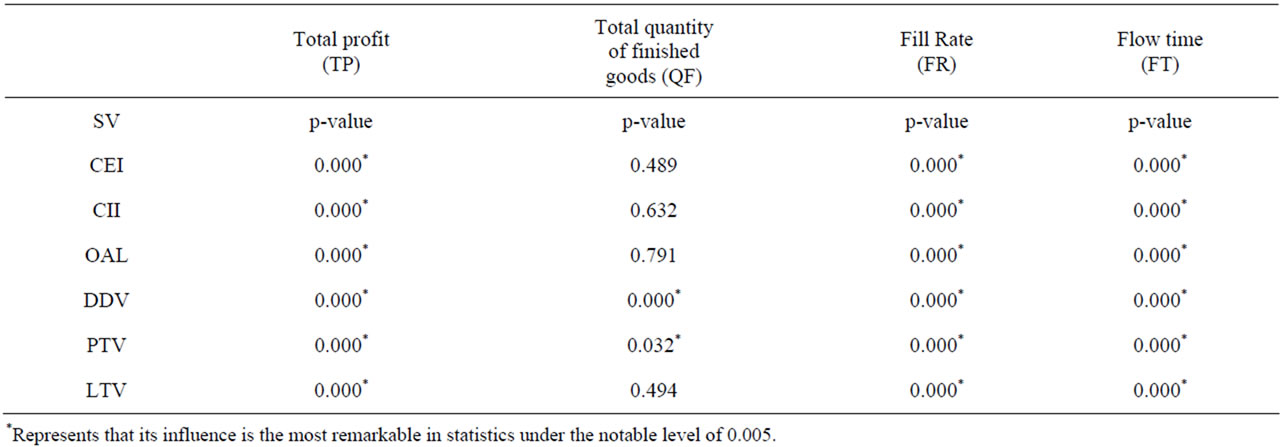
Table 5. Variance analysis results.
0.05, which expresses they have remarkable influence on fill rate, and the order grace level also has significant influence on it; as for the three variables of “uncertainty” (demand variable, processing time variable and lead time of material/part variable), all of them influence the fill rate notably.
In the part of external influence coefficient (CEI), the fill rate is higher in the situation of low-degree external influence coefficient (CIE = L1) than the high-degree external influence coefficient (CEI = L2) because of the flat demand curve and the relative low highest point of curve under the condition of low-degree external influence coefficient, hence the fill rate is high.
Seen from the results of simulation experiment, the fill rate is higher in the situation of low-degree internal influence coefficient (CII = L1) than high-degree internal influence coefficient (CII = L2). Because the demand curve is flat, and the highest point of curve is low relatively, the fill rate is high.
In the part of order grace level (OAL), the results of simulation experiment show that the fill rate is higher in the situation of high order grace level (OAL = L2) than low order grace level (OAL = L1). The reason is that the order delivery is short in the situation of low order grace level, which increases the probability of orders delay delivery, therefore the fill rate is naturally low.
In aspect of demand variability (DDV), there is higher fill rate on the condition of low variability (DDV = L1) than high variability (DDV = L2) in basis of the results of simulation experiment. The demand changes greatly under the condition of high variability. When the demand is large, there is a high probability to deliver orders late, so the fill rate is low.
In aspect of processing time variability (PTV), the results of simulation experiment exhibit that the fill rate is higher under the condition of low variability (PTV = L1) than high variability (PTV = L2). The reason is that the change of processing time is large in the situation of high variability. That the processing time is elongated has compact on the orders waiting in temporary storage areas of every operation are influenced, and it’s the probability of late delivery order that increases. Therefore the fill rate is also low.
In aspect of lead time variability (LTV), the fill rate is higher in the situation of low variability (LTV = L1) than high variability (LTV = L2) displayed by the results of simulation experiment. The change of lead time is large on the condition of high variability. When the lead time is elongated, the production will be delayed for lack of materials/parts, and then the orders waiting in temporary storage areas of every operation are influenced, which increases the probability of orders delivery late, so the fill rate is low.
5.4. Flow Time (FT)
Seen from the analysis on the variance of flow time, the p values of external influence coefficient (CEI) and internal influence coefficient (CII) are much less than 0.05, which expresses they have remarkable impact on flow time; but the order grace level has no significant influence on it; as for the three variables of “uncertainty” (demand variable, processing time variable and lead time of material/part variable), all of them influence the flow time notably.
In terms of external influence coefficient (CEI), generally speaking, the flow time is shorter on the condition of low-degree external influence coefficient (CEI = L1) than high-degree external influence coefficient (CEI = L2) shown as Table 5. Under the condition of low-degree external influence coefficient, the demand curve is flat and the highest point of curve is low relatively, so the flow time is short.
In terms of internal influence coefficient (CII), the results of simulation experiment shows that the flow time is short in the situation of low-degree internal influence coefficient (CII = L1) than high-degree internal influence coefficient (CII = L2). Because the demand curve is flat, and the highest point of curve is low relatively under the condition of low-degree internal influence coefficient, the flow time is short.
In terms of demand variability (DDV), generally speaking, there is shorter flow time on the condition of low variability (DDV = L1) than high variability (DDV = L2). The demand changes greatly under the condition of high variability, thus the flow time increases.
In terms of processing time variability (PTV), the results of simulation experiment exhibit that the flow time is shorter under the condition of low variability (PTV = L1) than high variability (PTV = L2). The reason is that the change of processing time is large in the situation of high variability, so the flow time increases.
In terms of lead time variability (LTV), the flow time is shorter in the situation of low variability (LTV = L1) than high variability (LTV = L2) displayed by the results of simulation experiment. Because the lead time is not steady in the situation of high variability, and the production will be delayed for lack of materials/parts when the lead time is elongated, consequently the flow time is added.
According to the results and analysis of this example and the influence degree of each experimental variables on every performance indexes, the outcome is shown as Table 5.
steady in the situation of high variability, and the production will be delayed for lack of materials/parts when the lead time is elongated, consequently the flow time is added.
6. Acknowledgements
This work was supported by Humanity and Social Science Youth foundation of Ministry of Education of China (No:11YJCZH054), Soft Scientific Research in the general project of Hunan Science and Technology Bureau (No: 2011ZK3031), Social Science foundation of Hunan Province (11YBA099), Scientific Research in the general project of Hunan Provincial Education Department of China (No: 11C0439) and Hunan University of Technology Research Project (No: 2011HSX05, No: 2011HS X18).
REFERENCES
- B. A. Pastenack, “Optimal Pricing and Returns Policies of Perishable Commodities,” Marketing Science, Vol. 4, No. 4, 1985, pp. 166-176. doi:10.1287/mksc.4.2.166
- Kurawarwala and Matsuo, “A System Modeling Framework for the Strategic Supply Chain Management of Food Supply Chains,” Journal of Food Engineering, Vol. 11, No. 6, 2005, pp. 351-364.
- T. Higuchi and M. D. Troutt, “Dynamic Simulation of the Supply Chain for a Short Life Cycle Product Lessons from the Tamagotchii Case,” Computers & Operations Research, Vol. 31, No. 7, 2004, pp. 1097-1114. doi:10.1016/S0305-0548(03)00067-4
- X. H. Xu, “Inventory Management and Operation Strategy of Short-Life-Cycle Product,” Material Press, China, 2007.
- L. J. Ding, G. P. Xia and J. Ge, “Supply Chain Coordination with Contract under Twice Producing and Ordering Model,” Journal of Management Sciences in China, Vol. 7, No. 4, 2004, pp. 24-32.
- B. Liu, “The Coordination Mechanisms and Modeling of Supply Chain for a Short-Life-Cycle Product,” Ph.D. Thesis, Nanjing University of Aeronautics and Astronautics, Nanjing, 2005.
- T. P. Zhang and J. H. Jiang, “Construction of Three-Tier Supply Chain Performance Evaluation Index System,” Seeker, Vol. 9, No. 6, 2010, pp. 38-40.
- S. J. Li, Z. B. Zhu and L. H. Huang, “Supply Chain Coordination and Decision Making under Consignment Contract with Revenue Sharing,” International Journal of Production Economics, Vol. 12, No. 1, 2009, pp. 88-99. doi:10.1016/j.ijpe.2008.07.015
- R. Mark and F. M. Frascatore, “Long-Term and Penalty Contracts in a Two-Stage Supply Chain with Stochastic Demand,” European Journal of Operational Research, Vol. 18, No. 6, 2008, pp. 147-156. doi:10.1016/j.ejor.2006.10.056
- J. Y. Wang, R. Q. Zhao and W. S. Tang, “Supply Chain Coordination by Single-Period and Long-Term Contracts with Fuzzy Market Demand,” Tsinghua Science and Technology, Vol. 14, No. 2, 2009, pp. 218-224. doi:10.1016/S1007-0214(09)70033-1