Positioning
Vol.2 No.1(2011), Article ID:3891,14 pages DOI:10.4236/pos.2011.21003
Point Selection for Triangular 2-D Mesh Design Using Adaptive Forward Tracking Algorithm
![]()
Digital Signal processing Research Lab, Department of Eelectrical and ComputerEengineering, Isfahan University of Technology, Isfahan, Iran.
Email: n_borjian2002@yahoo.com, {fattahi, sadri}@cc.iut.ac.ir.
Received November 27th, 2010; revised December 10th, 2010; accepted January 10th, 2011.
Keywords: Motion Estimation, Optical Flow, Pixel-Based, Block-Based-Region-Based, Mesh-Based, Adaptive-Forward Tracking, Polygon Approximation, Content-Based Mesh Structure, Triangulation, Affine Compensation, Mesh Refinement
ABSTRACT
Two-dimensional mesh-based motion tracking preserves neighboring relations (through connectivity of the mesh) and also allows warping transformations between pairs of frames; thus, it effectively eliminates blocking artifacts that are common in motion compensation by block matching. However, available uniform 2-D mesh model enforces connectivity everywhere within a frame, which is clearly not suitable across occlusion boundaries. To overcome this limitation, BTBC (background to be covered) detection and MF (model failure) detection algorithms are being used. In this algorithm, connectivity of the mesh elements (patches) across covered and uncovered region boundaries are broken. This is achieved by allowing no node points within the background to be covered and refining the mesh structure within the model failure region at each frame. We modify the occlusion-adaptive, content-based mesh design and forward tracking algorithm used by Yucel Altunbasak for selection of points for triangular 2-D mesh design. Then, we propose a new triangulation procedure for mesh structure and also a new algorithm to justify connectivity of mesh structure after motion vector estimation of the mesh points. The modified content-based mesh is adaptive which eliminates the necessity of transmission of all node locations at each frame.
1. Introduction
Motion estimation is an important part of any video processing system and is divided as 2-D motion estimation and 3-D motion estimation.
2-D motion estimation has a wide range of applications; including video compression, motion forward tracking, sampling rate conversion, filtering and so on. Depending on the intended applications for the resulting 2-D motion vectors, motion estimation methods can be very different. For example, for computer vision applications, the 2-D motion vectors will be used to deduce 3-D structure and motion parameters [1].
On the other hand, for video compression applications, the estimated motion vectors are used to produce a motion compensated prediction of a frame to be coded from a previously coded reference frame. The ultimate goal is to minimize the total bits used for coding the motion vectors and the prediction errors.
In motion tracking, the estimated motion vectors are used to predict position an object in next frame and tracking it in sequencing video images [2,3].
In this paper, we are concerned with methods of 2-D motion estimation and implementation one of them in motion tracking.
All the motion estimation algorithms (2-D) are based on temporal changes in image intensities (color). In fact, the observed 2-D motions based on intensity changes may not be the same as the actual 2-D motion. To be more precise, the velocity of observed or apparent 2-D motion vectors is referred to as optical flow. Optical flow can be caused not only by object motions, but also camera movements or illumination condition changes. In this paper, we define optical flow and its equation which imposes a constraint between image gradients and flow vectors [4]. This is a fundamental equality that many motion estimation algorithms are based on.
A key problem in motion estimation is how to parameterize the motion field. A 2-D motion field resulting from a camera or object motion can usually be described by a few parameters. However, there are typically multiple objects in the imaged scene that move differently. Therefore, a global parameterize model which assumes all objects in the scene have equally motion and estimates a vector motion for every scene or any frame is usually inadequate. It is suitable if only the camera is moving or image scene contains a single moving object with a planar surface. This method is feature-based and uses correspondences between pair of selected feature points in two video frames.
The most direct and unconstrained approach is to specify the motion vector at every pixel. This is called pixelbased representation. Such a representation is universally applicable, but it requires the estimation of a large number of unknowns (twice the number of pixels). In addition to, it requires special physical constraints to correct estimation [5-7].
For scenes containing multiple moving objects, it is more appropriate to divide an image frame into multiple regions, so that the motion within each region can be characterized well by a parameterized model. This is known as region-based motion representation. It consists of a region segmentation map and several sets of motion parameters (one for each region). The difficulty with such an approach is that one does not know in advance which pixels have similar motions. Therefore, segmentation and estimation must be accomplished iteratively, which requires intensive computations that may not be feasible in practice [8].
One way to reduce the complexity associated with region based motion representation is by using a fixed partition of the image domain into many small blocks. As long as each block is small enough, the motion variation within each block can be characterized well by a simple model and the motion parameters for each block can be estimated independently. This brings us to the popular block-based representation.
The simplest version models the motion in each block by a constant translation, so that the estimation problem becomes that of finding one motion vector for each block. This method provides a good compromise between accuracy and complexity and has found great success in practical video coding systems. One main problem with the block-based approach is that it dose not impose any constraint on the motion transition between adjacent blocks. The resulting motion is often discontinuous across block boundaries, even when the true motion field is changing smoothly from block to block [4,9].
One way to overcome this problem is by using a mesh-based representation, in which the underlying image frame is partitioned into no overlapping polygonal elements. The motion field over the entire frame is described by the motion vectors at the nodes (corners of polygonal elements) only and the motion vectors at the interior points of an element are interpolated from the nodal motion vectors.
This representation induces a motion field that is continuous every where. It is more appropriate than the blockbased representation over interior regions of an object which usually undergo a continuous motion, but it fails to capture motion discontinuities at object boundary; for example, when occlusion or overlapping to objects occurs.
Adaptive schemes such as adaptive block-matching [10] or adaptive mesh [11] that allow discontinuities when necessary are needed for more accurate motion estimation.
In this paper, we present the general methodologies for 2-D motion estimation and evaluate advantages and defects of them. In the following, we focus on the mesh algorithm and present a new adaptive mesh algorithm to forward motion tracking.
2-D mesh model is a method for motion tracking which allows spatial transformations and preserves neighboring relations between elements. This method tracks the motion by transmissions of the points in the elements that are computed from an estimated motion field [11,12].
2-D meshes can be classified as uniform (regular) meshes with equal size for elements [13], and nonuniform (hierarchical or content-based) ones that the size of elements is adapted to particular scene content [14-18]. The elements in the regular mesh may overlap within the subsequent frames of the image while a nonuniform mesh is adapted on the boundary of the objects. Furthermore, a uniform mesh is not suitable when there were more than one type of motion in the scene [19,20].
In fact, Object tracking is monitoring the object position variations and tracking it during a video sequence for a perpendicular purpose. The success of forward tracking is closely related to how well we can detect occlusion and model failure regions and estimate the motion field in the vicinity of their boundaries. Motion compensation is necessary to determine points to be killed and the locations of the newly born points.
In this paper, we present an adaptive forward-tracking mesh procedure which in it, none of the points are allowed to locate in the background regions that will be covered in the next frame (BTBC regions) and the mesh within the model failure region(s) is redefined for subsequent tracking of these regions [21].
In addition to, we present the basics of adaptive mesh algorithm, estimation motion fields and BTBC region detection. Then, polygon approximation is reviewed. Next, we present a new, efficient, adaptive forwardtracking mesh design procedure that is employed to design the initial mesh.
In the following, a new triangulation method is proposed. Point motion estimation for the purposes of motion compensation and mesh tracking are implemented too, which are followed by a forward node tracking and mesh refinement algorithm.
Experimental results on the synthetic and simple images showed that the new presented adaptive forwardtracking mesh algorithm is successful in motion tracking. On the other word, the results shown in this paper are synthetic. But, in next step, this new algorithm must be tested on the real states consist of deformation or multiple objects scenes and results must be compared to other algorithms for tracking the object especially in presence the occlusion.
2. Optical Flow Equation
Consider a video sequencer whose luminance variation is represented by . Suppose an image point
  at time
  is moved to
  at time
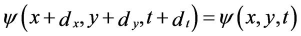
 . Under the constant intensity, the images of the same object point at different times have the same luminance value. Therefore:
 (1)
(1)
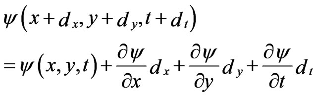
Using Taylor’s expansion, when ,
,  and
and  are small, we have:
 (2)
(2)
Combining Equations (1) and (2) yields:
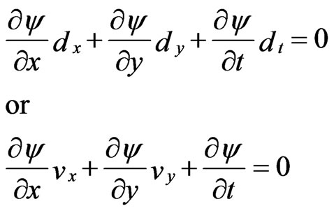 (3)
(3)
Where 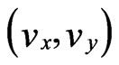 represents the velocity vector or flow vector. Equation (3) known as the “optical flow equation”. [22]
3. Pixel-Based Motion Estimation
In pixel motion estimation, one tries to estimate a motion vector for every pixel. Obviously, this scheme is ill-defined. If one uses the constant intensity assumption into two sequenced frame k and k + 1, for every pixel in the k frame, there will be many pixels in the k + 1 frame that have exactly the same image intensity. If one uses the optical flow equation instead, the problem exists again, because there is only one equation for two unknowns.
To circumvent this problem, there are in general four approaches:
First, one can use regularization techniques to enforce smoothness constraints on the motion field, so that the motion vector of a new pixel is constrained by those found for surrounding pixels. Second, one can assume that the motion vectors in a neighborhood surrounding each pixel are the same and apply the constant intensity assumption or the optical flow equation over the entire neighborhood.
Third, one can make use of additional invariance constraints; in addition to intensity invariance which leads to the optical flow equation. For example, one can assume that the intensity gradient is invariance under motion as proposed in [5-7].
Finally, one can also make use of the relation between the phase functions of the frame before and after motion [23].
4. Block-Based Motion Estimation
As we have seen, a problem with pixel-based motion estimation is that one must impose smoothness constraints to regularize the problem.
One way of imposing smoothness constrains on the estimated motion field is to divide the image domain into nonoverlapping small region which called “blocks” and assume that motion within each block can be characterized by a simple parametric model; for example, constant, affine or bilinear.
If the block is sufficiently small, then this model can be quite accurate.
Assume that  represents the image block ‘m’ and ‘M’ is number of blocks and K = {1,2,…,M}; partition into blocks should satisfy:
 = “entire image” and
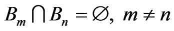
Theoretically, a block can have any polygonal shape. In practice, the square shape is commonly used; although the triangular shape can be used also and it is more appropriate when the motion in each block is described by an affine model.
Figure 1 illustrates the effect of several of the motion representation for a head-and-shoulder scene.
4.1. Block Matching Algorithm
In the simplest case, the motion in each block is assumed to be constant, that is, the entire block undergoes a translation. Therefore, the motion estimation problem is to find a single motion vector for each block. This type of algorithm is referred as the block matching algorithm [24].
Given an image block  in the anchor frame, the motion estimation problem is to determine a matching block
  in the target frame such that the error between
 (a)
(a)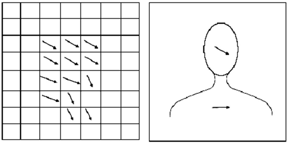 (b)
(b)
Figure 1. Different motion representation: (a) global (b) pixel-based (c) block-based (d) region-based.
these two blocks is minimized. (If motion is forward, anchor frame represents frame k and target frame represents k + 1 frame. Otherwise, if motion is backward, anchor frame represents frame k + 1 and target frame represents k frame.)
The displacement vector  between the spatial positions of these two blocks (in terms of center or a selected corner) is the motion vector of this block. In the other word,
  ,
,  in anchor frame is related to
  in target frame.
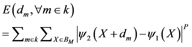
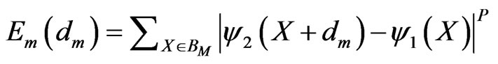
The most popular criterion for motion estimation is error function or the sum of he differences between the luminance values of every pair of corresponding points between the anchor frame  and the target frame
 . Under the blocking translational model, error equation can be written as:
 (4)
(4)
Which, p is a positive number. When p = 1, the error function (for every motion estimation algorithm) is called the “mean absolute difference”, and when p = 2, it is called “mean squared error”.
Because the estimated motion vector for a block affects the prediction error in that block only, one can estimate the motion vector foe each block individually by minimizing the prediction error accumulated over each block, which is:
 (5)
(5)
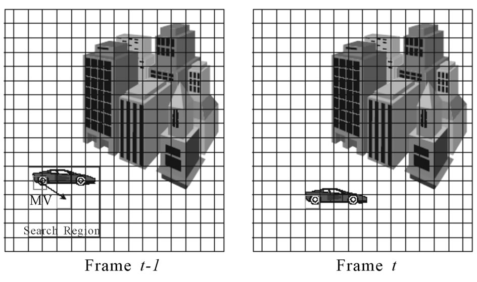
One way to determine  that minimize this error is by using exhaustive search. As illustrated in Figure 2, this scheme determines the optimal
  for a given block
  in the anchor frame by comparing it with all candidate blocks
  in the target frame within a predefined search region and finding the one with the minimum error. The displacement between the two blocks is the estimated motion vector.
But the exhaustive search algorithm requires a very large amount of computation. For a search range of  and a step size of 1 pixel, the total number of candidates is
 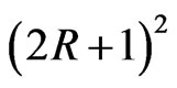 whit this algorithm. To speed up the search, various fast algorithms for block matching have been developed. The key to reducing the computation is reducing the number of search candidates. Various fast algorithms differ in the ways that they skip those candidates that are unlikely to have small error. The most important fast search algorithms are 2-D-log search method [25] and Three-step search method [26].
In the block matching algorithm, one assumes that the motion in each block is constant. But, if it is necessary to characterize the motion in each block by a more complex model, deformable block matching algorithm can be used.
 (a)
(a)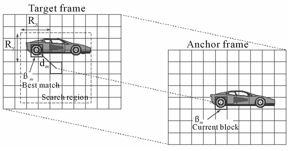 (b)
(b)
Figure 2. The search procedure for block-matching algorithm.
4.2. Deformable Block Matching Algorithm
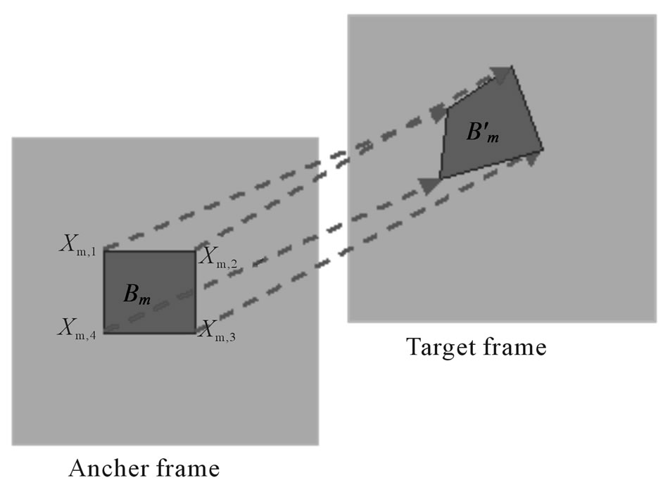
In the block matching algorithm introduced previously, each block is assumed to undergo a pure translation. This model is not appropriate for blocks undergoing rotation, zooming and so on. In general, a more sophisticated model such as the affine, bilinear or projective mapping can be used to describe the motion of each block. (Obviously, this will still cover the translation model as a special case.) With such model, a block in the anchor frame is in general mapped to a nonsquare quadrangle as shown in Figure 3. Therefore, the class of block-based motion estimation methods using higher order models is referred as deformable block matching algorithms [27-29].
In this algorithm, the motion vector at any point in a block is interpolated by using only motion vectors at the block corners (called nodes) [30].
Assume that a selected number of control nodes in a block can move freely and that the displacement of any interior point can be interpolated from nodal displacement. Let the number of control nodes be denoted by K and the motion vectors of the control nodes in  by
by . Then, the motion function over the block is described by:
 (6)
(6)
Equation (6) expresses the displacement at any point
 (a)
(a)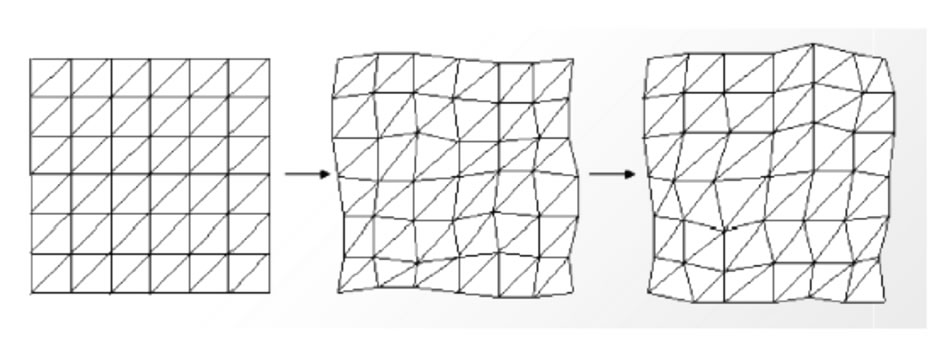 (b)
(b)
Figure 3. The deformable block-matching algorithm.
in a block as an interpolation of nodal displacements as shown in Figure 4.
With this model, the motion parameters for any block are the nodal motion vectors that can be estimated by minimizing the prediction error over this block, which is:
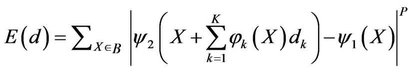 (7)
(7)
Because the estimation of nodal movements is independent from block to block, we omit the subscript ‘m’. The interpolation kernel 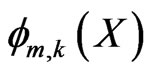 depends on the desired contribution of the control point k in
  to the motion vector at X. one way to design the interpolation kernels is to use the shape functions associated with the corresponding nodal structure [31]. To guarantee continuity across element boundaries, the interpolation kernel should satisfy:
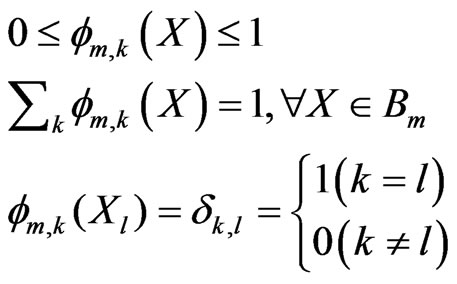 (8)
(8)
Standard triangular and quadrilateral elements are shown in Figure 5. The shape functions for the standard triangular element are:
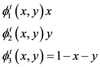 (9)
(9)
The shape functions for the standard quadrilateral element are:
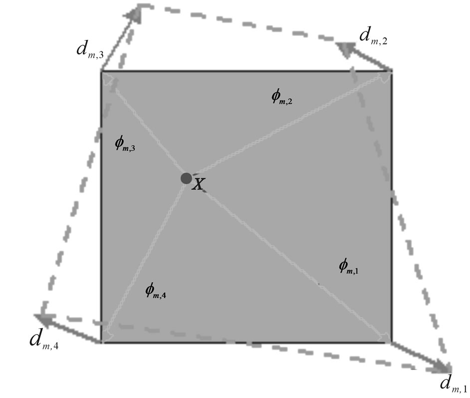
Figure 4. Interpolation of motion in a block from nodal motion vectors.
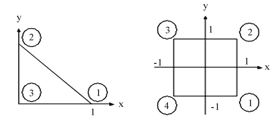
Figure 5. A standard triangular element and a standard quadrilateral element.
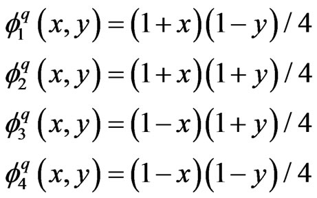 (10)
(10)
5. Mesh-Based Motion Estimation
With the block-based model used in either block-match-ing or deformable block-matching, motion parameters in individual blocks are independently specified. Unless motion parameters of adjacent blocks are constrained to very smoothly, the estimated motion field is often discontinuous and some times chaotic as illustrated in Figure 6.
One way to overcome this problem is by using mesh-based motion estimation. As illustrated in Figure 7, the anchor frame is covered by a mesh and the motion estimation problem is to find the motion of each node, so that the image pattern within each element in the anchor frame matches well with that in the corresponding deformed element in the target frame.
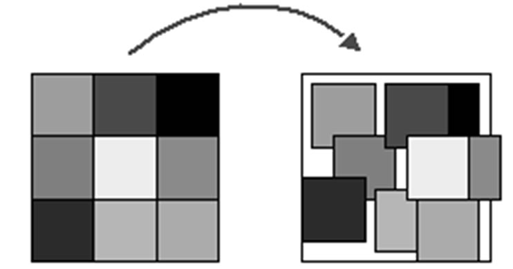
Figure 6. The blocking artifacts caused block-based motion estimation.
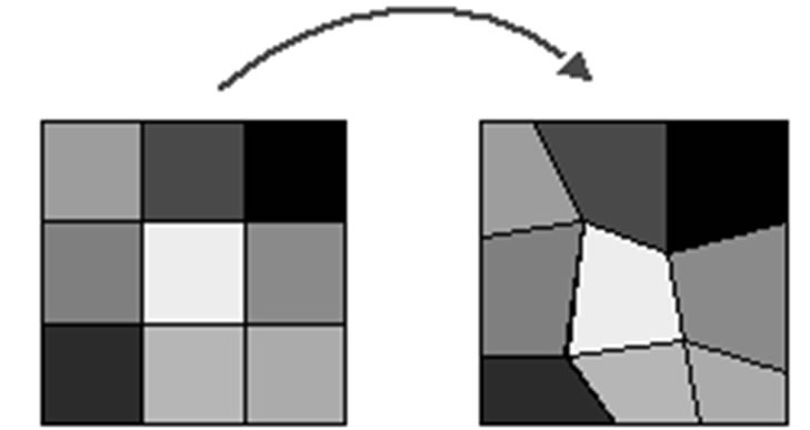
Figure 7. No artifact using mesh-based motion estimation.
The motion within each element is interpolated from nodal motion vectors, as long as the nodes in the target frame still form a feasible mesh. The mesh-based motion representation is guaranteed to be continuous and thus be free from the blocking artifacts associated with blockbased representation. Another benefit of mesh-based representation is that it enables continuous tracking of the same set of nodes over consecutive frames, which is desirable in applications requiring object tracking.
As shown in Figure 7, one can generate a mesh for initial frame and then estimate the nodal motions between every two frames. At each new frame, the mesh generated in the previous step is used, so that the same set of nodes is tracked over all frames. This is not possible with block-based representation, because it requires that each new frame be reset to a partition consisting of regular blocks.
As said above, in mesh-based motion representation, the underlying image domain in the anchor frame is partitioned into non overlapping polygonal elements. Each element is defined by a few nodes and links between the nodes as shown in Figure 8. The motion field over the entire frames is described by motion vectors at the nodes only. The motion vectors at the interior points of an element are interpolated from the motion vectors at the nodes of this element. In addition to, the nodal motion vectors are constrained so that the nodes in the target frame still form a feasible mesh with no overlapped elements.
Let the number of elements be denoted by M and the motion vector of the node k in  by
by . The number of nodes defining each element is K. Then, the motion function over the element
  is described by:
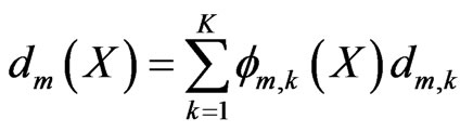 (11)
(11)
With the mesh-based motion representation, the motion parameters include the nodal motion vectors. To estimate them, we can again use an error-minimization approach such as:
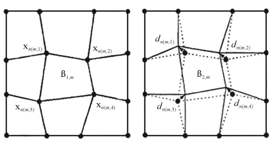
Figure 8. Illustration of mesh-based motion representation using a quadrilateral mesh.
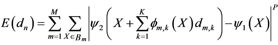 (12)
(12)
The , is nodal motion vector in node ‘n’.
The accuracy of mesh-representation depends on the number of nodes. A very complex motion field can be reproduced when a sufficient number of nodes are used. To minimize the number of nodes required, the mesh should be adapted to the image scene so that the actual motion within each element is smooth. In real-world video sequences, there are often motion discontinuities such as occlusion at object boundaries. A more accurate representation would use separate meshes for different object or adapt the mesh in every two sequence frame. This algorithm is referred as “adaptive mesh algorithm”.
6. Adaptive Mesh
In the following, we present the basics of adaptive mesh algorithm.
6.1. Adaptive Mesh Concept
Standard mesh models enforce continuity of motion across the whole frame and it is not desired when multiple motion and occlusion regions are presented [11,12]. We introduce the adaptive mesh concept to overcome this fundamental limitation. Consider a moving elliptical object, which is shown in Figure 9. Assume that the elliptical object is translating to the right, thus there are two types of motion: motion to the right that is assigned to the BTBC region, and to the left that is assigned to the UB region. The BTBC region in frame k should be covered in frame k + 1 completely.
6.2. Estimation Motion Field
Estimation motion field algorithm estimates motion vectors at each pixel independently from an optical flow field using method of Horn-Schunck [32]. An optical flow-based method is better than for example block matching method, because the former yields smoother motion fields, which are more suitable for parameterization
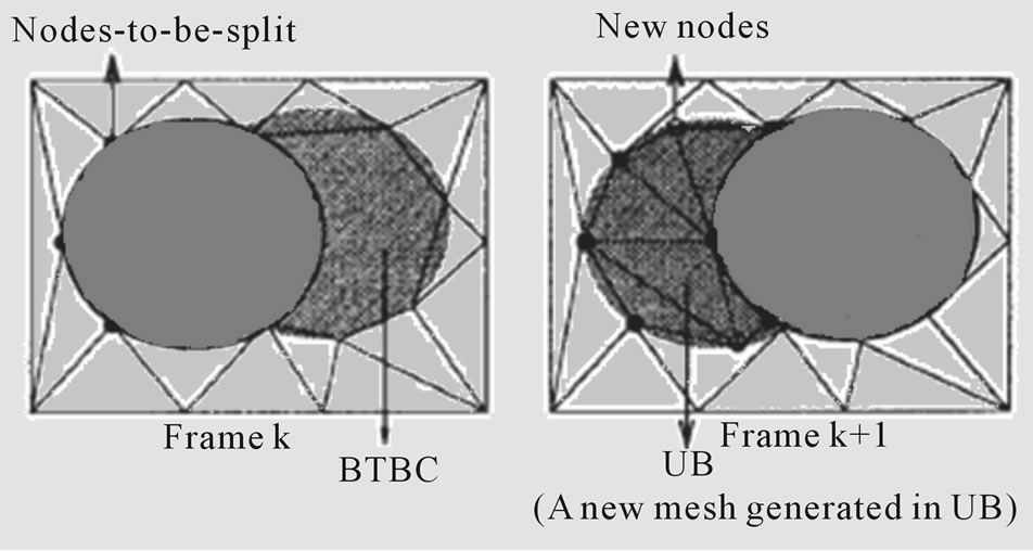
Figure 9. Adaptive mesh concept.
[33]. In [34] Lucas and Kanade present another method for motion estimation based on split-and-merge scheme.
In this paper, we use a point scheme to solve the optical flow equation [35]. Assume a block such as Figure 10 for every pixel and compute the partial derivations based on according to Equation (13).
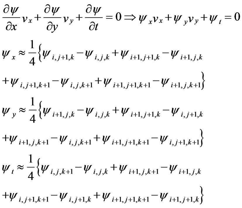 (13)
(13)
We require an extra condition to solve the optical flow equation which minimizing the gradient or laplacian relations according Equation (14) to smooth the motion field can be used.
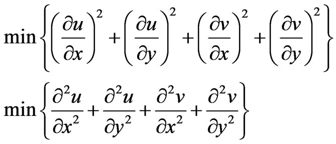 (14)
(14)
If all objects in the scene move together, only one ![]() and one
and one ![]() will exit for scene. Therefore, minimizing to smooth the motion filed can be used on the summation square optical equations in all pixels.
will exit for scene. Therefore, minimizing to smooth the motion filed can be used on the summation square optical equations in all pixels.
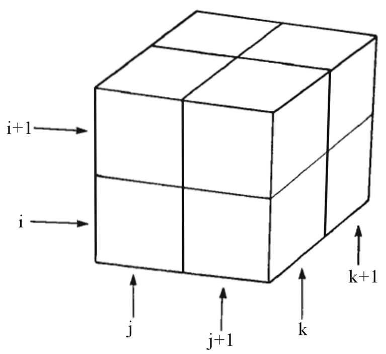
Figure 10. The block to compute partial derivations in every pixel.
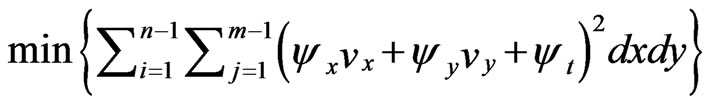 (15)
(15)
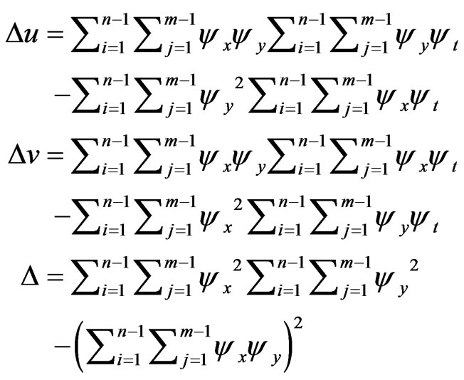 (16)
(16)
6.3. BTBC Region Detection
We introduce the following algorithm to BTBC detection that is used in [11,12]:
1) Calculate the frame difference and determine the change region by thresholding and processing as follows:
a) Filtering by the median filter with a 5 × 5 size.
b) Three times morphological closing operations with a 3 × 3 size and then three times morphological opening operations with the same size.
c) Eliminate small regions, which are smaller than predetermined size for example 25 pixels.
2) Estimate motion field from frame k to frame k + 1.
3) Compensate the motion for frame k from frame k + 1 to compute figurative frame  using the motion field.
4) If the difference between  and
and  is greater than a predefined threshold, then the pixel
  is labeled as an occlusion pixel. That is:
If 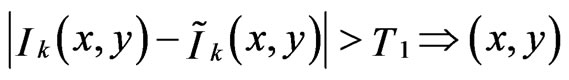 is occluded (17)
The amount of threshold (T1) is depend on scene and can be defined by any matter. For example, half the biggest different between the pixels of k frame and the pixels of k + 1 frame or the average of different between all pixels of k frame and k + 1 frame can be used. However, T1 should be determined experimentally.
Figure 11 illustrates the BTBC region detection for two scenes.
6.4. Polygon Approximation
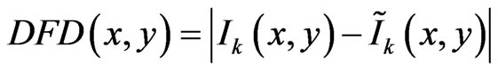
Polygon approximation can be used when the boundary of a region must be approximated by a set of points, so that it provides nearest approximation to the region with a few parameters. This simple approximation naturally fits with the boundaries of the region. See Figure 12 for more details. The used polygon approximation algorithm
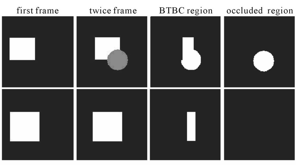
Figure 11. BTBC region detection.
is similar to that proposed in [11,36], as follows:
1) Find two pixels on the boundary of the region (1 and 2), which have maximum distance from each other. The line drawn between these two points is called the main axis.
2) Find the two points on the boundary (3 and 4) in two opposite sides of the axis which have the largest perpendicular distance from the main axis. These four points are named the initial points.
3) Now, there are four segments; 1-3, 3-2, 2-4 and 4-1. Consider segment 1-3. Draw a straight line from point 1 to the point 3. Detect every point on the boundary between 1 and 3 and every point in the area between the boundary and the straight line. If the maximum perpendicular distance between the straight line and every point on the boundary is below a certain threshold and the pixels that are in the area between the boundary and the straight line is less than 5% of total pixels of the region, then no new points need to be inserted on this segment of the boundary. If, however both criteria are not satisfied simultaneously, a new point on the boundary must be inserted at the pixel with the maximum distance from the straight line, and this procedure is repeated until no new points are needed within each new segment.
4) Repeat step 3 for three remaining segments.
Results of algorithm for several desired regions are shown in Figure 13. The criterion of stopping the algorithm can be the predetermine number of points on the boundary. If number of inserted points on the boundary is exceeded on upper criterion (say, 64), the algorithm is stopped. But, this number of points is not needed in practice. The algorithm is able to expansion up 128 or 256 points simply.
6.5. Selection the Points for Triangular 2-D Mesh Design
In the following, we propose a new, computationally efficient algorithm to select the points for 2-D triangular mesh design. This algorithm incorporates a nonuniform mesh, so that the density of points is proportional to the local motion activity and the mesh boundaries match with object boundaries. Thus, the points are located on spatial edges or pixels with high spatial gradient. This is shown in Figure 14. Then, a triangulation procedure is performed using the selected points. The algorithm is as follows [37]:
1) Approximate the region of object by polygon approximation.
2) All pixels except of the BTBC region are labeled unmark. Compute DFD average for all unmarked pixels by the following expression:
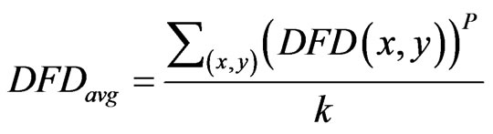 (18)
(18)
Which
 (19)
(19)
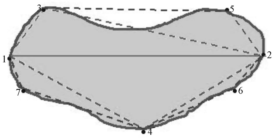
Figure 12. Polygonal approximation.
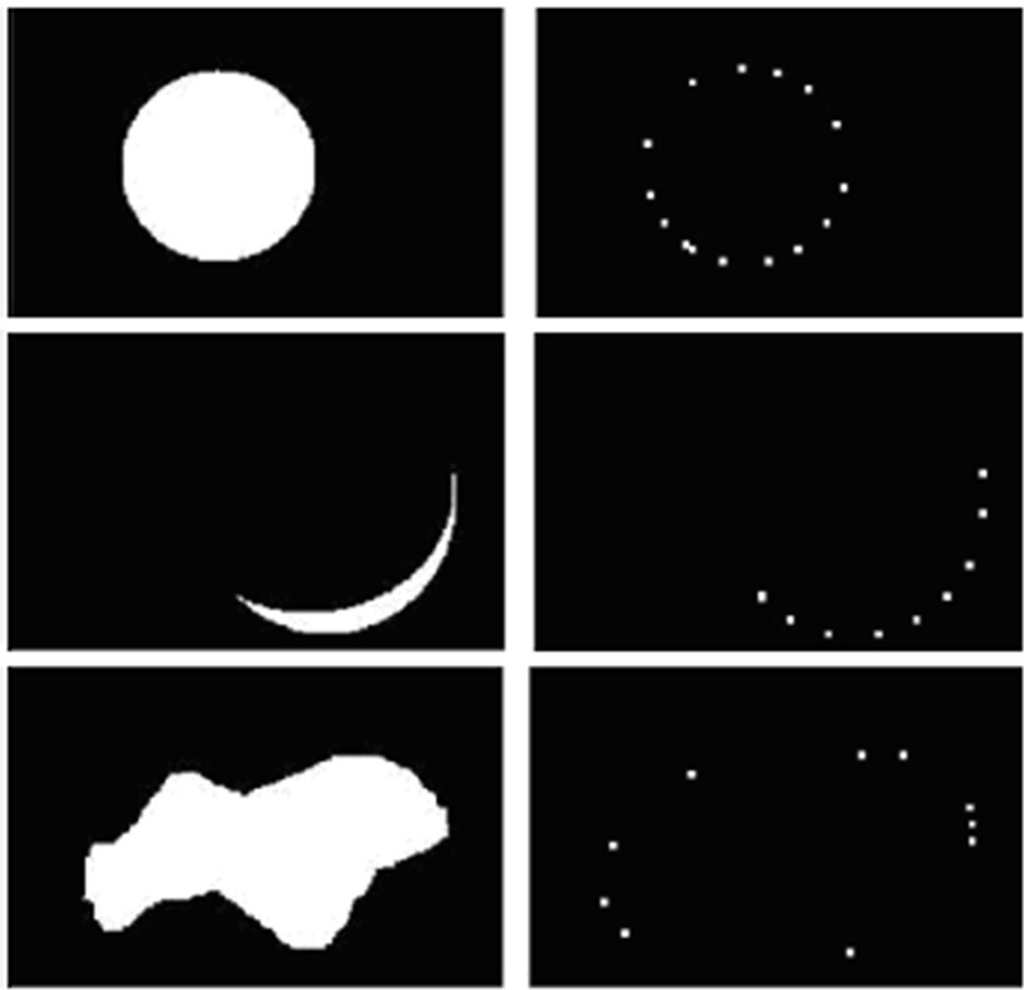
Figure 13. Result of algorithm polygonal approximation.

Figure 14. Selection the points for mesh design.
And k is number of unmarked pixels and p can be selected equal 1 or 2.
3) Grow a circle about every point that is gained from polygon approximation until  in this circle is greater than DFD average. Label all pixels within the circle as “marked.”
4) Label the BTBC region.
5) Compute a cost function for each unmarked pixel by:
 (20)
(20)
where  and
and  are partial derivations.
6) Select an unmarked pixel, which has highest cost function 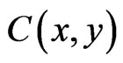 and consider a circle region with a predefined radius about it. If there is no other marked pixel in the circle, label the new pixel.
7) Grow a circle about it similar to step 3. Stop growing when marked region is merged the other marked region even the condition in step 3 is not satisfied.
8) Repeat step 6 until a desired number of points are selected.
Figure 15 shows the result of procedure. It consists of grown regions for a square, which has moved to the right.
6.6. Triangulation
We propose a fast and simple algorithm for triangulation, called star-polygon method. The algorithm is as follows:
1) Consider point M of set point of the mesh.
2) Find the nearest neighbor point over the point M.
3) Find the nearest neighbor point under the point M. See Figure 16.
4) Divide the plan in two parts by a vertical line passed through M.
5) Consider all points at the right half plan. If two points are on the same line passing through M, keep the point that is closer to M and cancel the other. Repeat this step until no two points are located in the same line passing through M.
6) Also repeat step 5 for all points at the left half plan.
7) Connect M to remained points. This makes a star on the graph.
8) Scan all radiuses of star clockwise, from top to bottom and make a triangle between successive radiuses until the polygon of point M become complete.
9) Repeat the algorithm for every point of set point of the mesh.
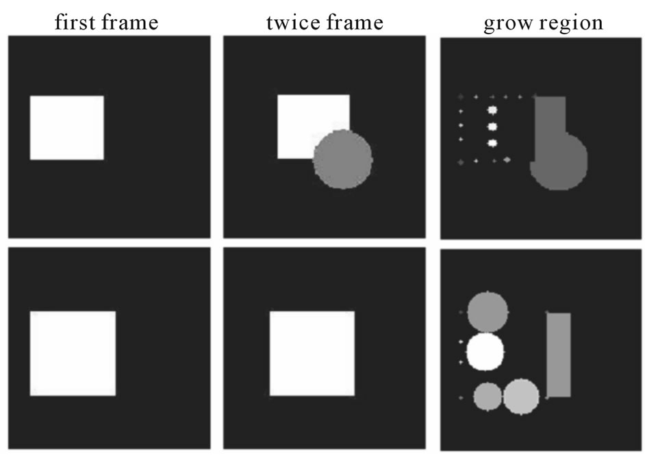
Figure 15. Result of algorithm selection points.
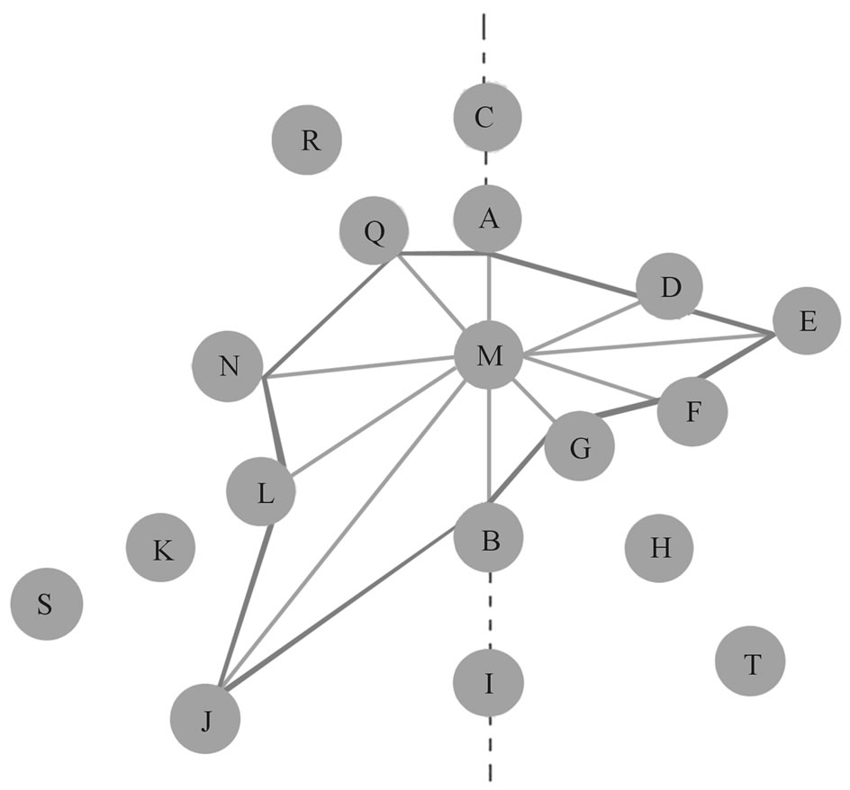
Figure 16. Star-polygon triangulation.
The triangles should not be overlapped. Thus, we use Delaunay triangulation condition to build triangles with no overlaps. Delaunay triangulation is a kind of triangulation, which has the following specification: if a circle is circumscribed triangle, no other points of the mesh are within the circle. This is shown in Figure 17.
Result of algorithm drawing a circle that is circumscribed desire triangle is shown in Figures 18 and 19 illustrate the result of algorithm triangulation for several desired set of points too.

Figure 17. Delaunay triangulation.
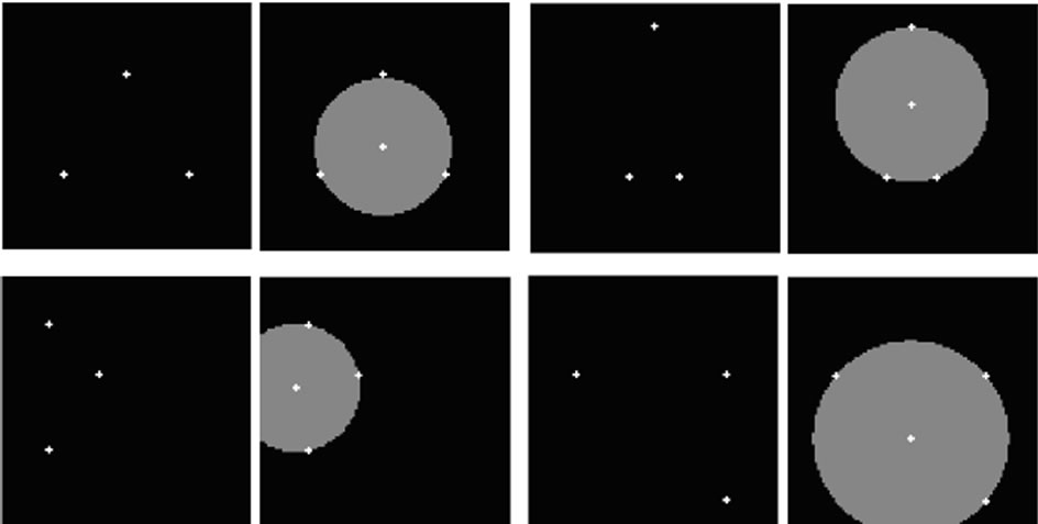
Figure 18. drawing the circle that is circumscribed the desired triangle.
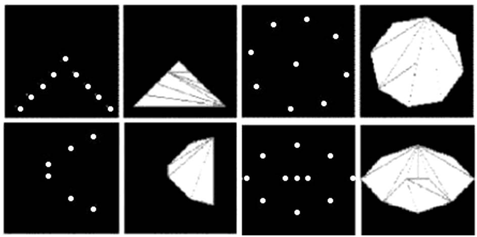
Figure 19. Result of algorithm triangulation.
6.7. Forward Tracking
Forward tracking has the following steps:
1. Motion vector estimation for selected points.
2. Affine motion compensation.
3. Model failure region detection.
4. Refinement of the mesh structure.
6.7.1. Motion Vector Estimation for Selected Points
Motion vector estimation for selected points can be accomplished using the computed motion field in BTBC detection part. But, it is possible that estimated motion vectors are inconsistent in the sense that they do not preserve the connectivity of the mesh structure. This is shown in Figure 20.
Also, following steps ensures that the connectivity of the mesh structure is fulfilled:
1) Consider point  and all points connected to it.
2) Find the points mapped from previous frame to the next and name them .
.
3) Compute virtual point  by:
by:
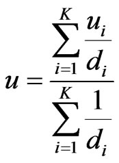 and
and 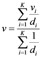 (21)
(21)
where  is motion vector of virtual point
  and
and 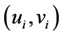 is motion vector of every point
  connected to
  and
and  is the distance between them.
4) Build a polygon using the method that is similar to triangulation part by virtual point  and other
  points.
5) If is inside this polygon, select this point otherwise select virtual point
 .
.
6.7.2. Affine Motion Compensation
Every pixel  in frame k is related to a pixel
  in frame k + 1 similar to Figure 21. The relations in affine motion compensation are:
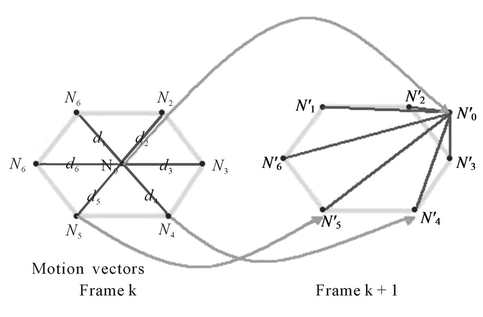
Figure 20. Non connectivity of the mesh structure.
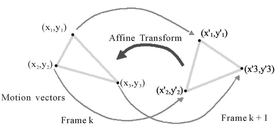
Figure 21. Affine motion compensation.
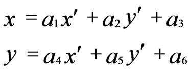 (22)
(22)
Accordingly affine motion compensation algorithm is as follows:
1) Compute the affine parameters for a triangular element by:
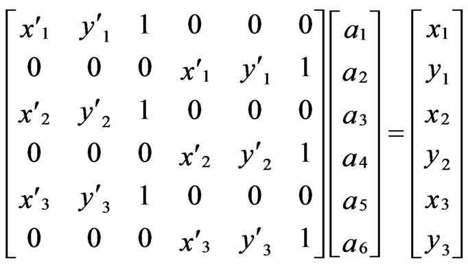 (23)
(23)
2) Compensate all points in this element by computed parameters and (22).
3) Repeat steps 1 and 2 for all triangular elements to compute figurative .
.
6.7.3. Model Failure Region Detection
Model failure region is detected by thresholding the difference between  and
and . The following relation must be satisfied:
 (24)
(24)
Similar to T1, The threshold T2 is depend on scene and determined experimentally too. For example, the relation T2 = T1 can be a selection.
6.7.4. Refinement of the Mesh Structure
All  points refine mesh structure. But if a point is located in model failure region or BTBC region between k + 1 and k + 2 frames, that point has to be canceled because such a point has not a true motion vector. Also a set of new points is located in model failure region.
The region recognized as object area is used for next frame.
Results of adaptive forward-tracking mesh algorithm are shown in Figure 22 and Figure 23.
The first row shows three successive frames produced by motion of camera. The second row includes the BTBC and occlusion regions between frames 1 and 2 and result of cost function. The third row shows the mesh structure, affine compensation and . Finally, the fourth row consists of model failure region, BTBC between frames 2 and 3, and at last predicted region of object in the next frame.
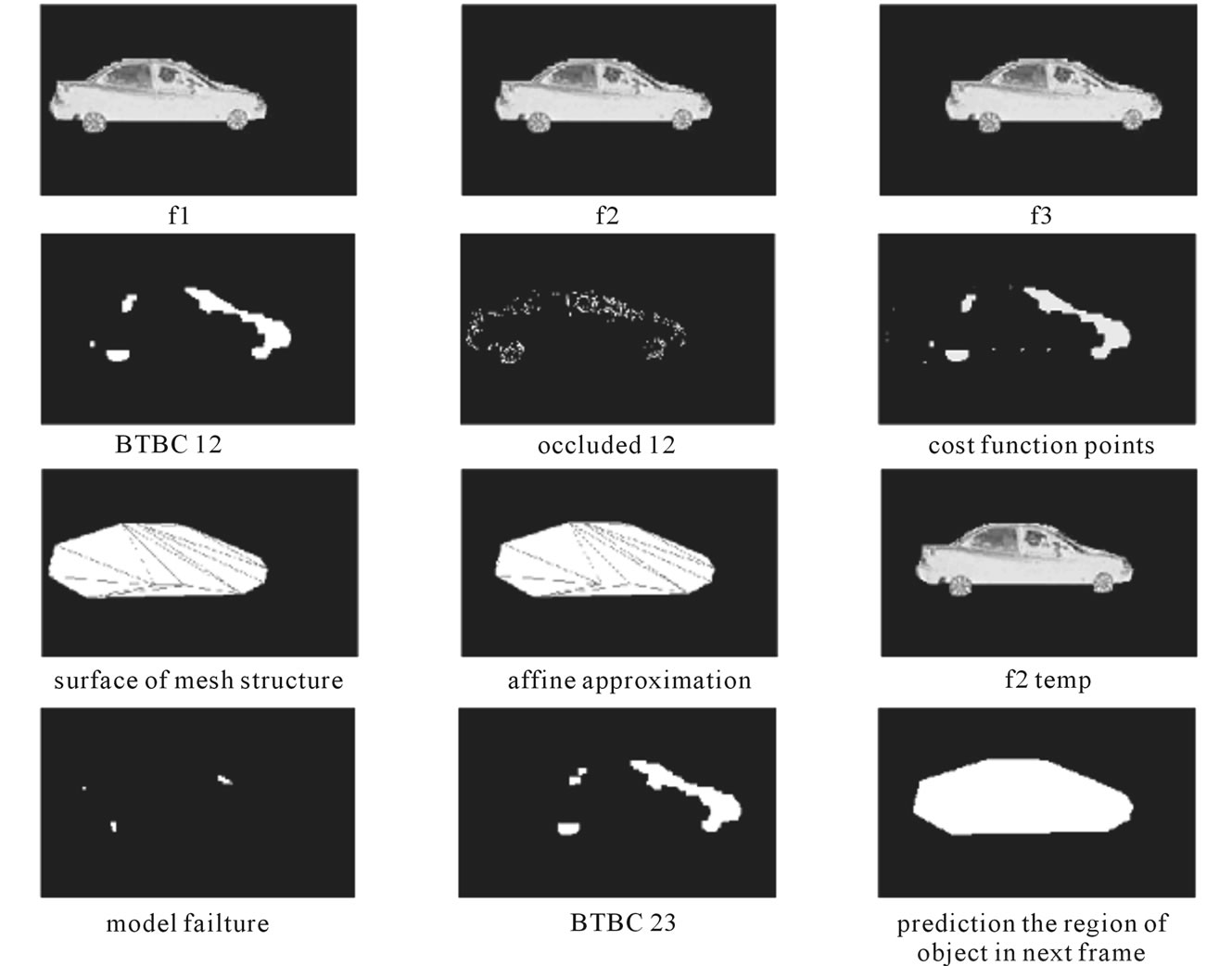
Figure 22. Results of adaptive forward tracking mesh algorithm (1).
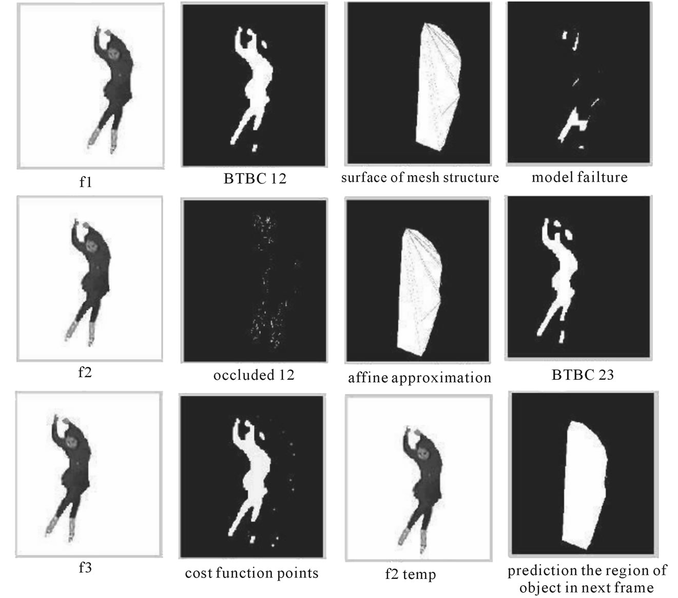
Figure 23. Results of adaptive forward tracking mesh algorithm (2).
7. Conclusions
In this paper, we investigated motion tracking algorithms especially mesh-based motion estimation. We implemented optical flow for motion field estimation and polygon approximation. We also modified content-based mesh method in mesh design part and proposed a new triangulation method to determine the mesh structure. Also, we proposed a procedure to ensure the connectivity of mesh structure. In addition we implemented affine compensation and refinement of the mesh structure procedures. Simulation results on the synthetic images show that the performance of modified and proposed parts in algorithm is acceptable.
REFERENCES
- J. K. Aggarwal and N. Nandhahumar, “Computation of Motion from Sequences of Images,” Proceeding of the IEEE, Vol. 76, 1988, pp. 917-935. doi:10.1109/5.5965
- H. G. Musmann, P. Pirsch and H. J. Grallert, “Advances in Picture Coding,” Proceeing of the IEEE, Vol. 73, 1985, pp. 523-548. doi:10.1109/PROC.1985.13183
- C. Stiller and I. Konrad, “Estimating Motion in Image Sequences,” IEEE Signal Processing Magazine, Vol. 16, 1999, pp. 70-91. doi:10.1109/79.774934
- Y. Wang, J. Ostermann and Y. Zhang, “Video Processing and Communications,” Chapter 1, Prentice Hall, New Jersey, 2002.
- H. H. Nagel, “Displacement Vectors Derived from Second-Order Intensity Variations in Images Sequences,” Computer Graphics and Image Processing, Vol. 21, 1983, pp. 85-117. doi:10.1016/S0734-189X(83)80030-9
- A. Mitiche, Y. F. Wang and J. K. Aggarwal, “Experiments in Computing Optical Flow with Gradient-Based, Multiconstraint Method,” Pattern Recognition, Vol. 20, 1987, pp. 173-179. doi:10.1016/0031-3203(87)90051-3
- R. M. Haralick and J. S. Lee, “The Facet Approach to Optical Flow,” Image Understanding Workshop, 1993.
- Y. Wang, X. M. Hsieh, J. H. Hu and O. Lee, “Region Segmentation Based on Active Mesh Representation of Motion,” IEEE International Conference on Image Processing, 1995, pp. 185-188.
- B. Girod, “Motion Compensation: Visual Aspects, Accuracy, and Fundamental Limits,” Motion Analysis and Image Sequence Processing, 1993, pp. 126-152.
- M. Ghoniem and A. Haggag, “Adaptive Motion Estimation Block Matching Algorithms for Video Coding,” International Symposium on Intelligent signal Processing and Communication, IEEE, Vol. 6, 2006, pp. 427-430.
- Y. Altunbasak, A. Murat Tekalp, “Occlusion-ADAPTIVE, Content-Based Mesh Design and Forward Tracking,” IEEE, Transaction on Image Processing, Vol. 6, No. 9, 1997, pp. 1270-1280. doi:10.1109/83.623190
- Y. Altunbasak, A. Murat Tekalp, “Occlusion-Adaptive 2-D Mesh Tracking,” IEEE, Vol. 4, No. 1, 1996, pp. 2108-2111.
- M. Sayed, W. Badawy, “A Novel Motion Estimation Method for Mesh-Based Video Motion Tracking,” IEEE, Vol. 4, 2004, pp. 337-340.
- P. Beek, A. Murat Tekalp, “Hierarchical 2-D Mesh Representation, Tracking, and Compression for Object-Based Video,” IEEE, Transactions on Circuits and Systems for Video Technology, Vol. 9, No. 2, 1993, pp. 353-369. doi:10.1109/76.752101
- Y. Altunbasak, G. Al-Regib, “2-D Motion Estimation with Hierarchical Content-Based Meshes,” IEEE, 2001, pp. 1621-1624.
- N. Laurent, “Hierarchical Mesh-Based Global Motion Estimation, including Occlusion Areas Detection,” IEEE, 2000, pp. 620-623.
- Y. Wei, W. Badawy, “A New Moving Object Contour Detection Approach,” IEEE, International Workshop on Computer Architectures for Machine Processing, Vol. 3, 2003, pp. 231-236.
- S. A. Coleman, B. W. Scotney, “Image Feature Detection on Contents-Based Meshes,” IEEE, International Computer Image Processing, Vol. 1, 2002, pp. 844-847.
- J. Weizhao, P. Wang, “An Object Tracking Algorithm Based On Occlusion Mesh Model,” In: Proceeding First International Conference on Machine Learning and Cybernetics, Vol. 1, 2002, pp. 288-292.
- C. Toklu, “2-D Mesh-Based Tracking of Dformable Objects with Occlusion,” IEEE, Vol. 1, 1996, pp. 933-936.
- C. Toklu, “2-D Mesh-Based Synthetic Transfiguration of an Object with Occlusion,” IEEE, Vol. 4, 1997, pp. 2649-2652.
- T. Hai, “Optical Flow,” Image Analysis and Computer Vision, University of California.
- D. J. Fleet and A. D. Jepson, “Computation of Component Image Velocity from Local Phase Information,” International Journal of Computer Vision, Vol. 5, 1990, pp. 77- 104. doi:10.1007/BF00056772
- Y. Wang, “Motion Estimation for Video Coding,” Polytechnic University, Brooklyn, 2003.
- J. R. Jain, “Displacement Measurement and Its Application in Inter Frame Image Coding,” IEEE, transaction on image processing, Vol. 29, 1981, pp. 1799-1808.
- T. Koga, “Motion Compensated Inter Frame Coding for Video,” Telecommunication Conference, Vol. 3, 1981, pp. 1-5.
- O. Lee and Y. Wang, “Motion Compensated Prediction Using Nodal Based Deformable Block Matching,” Journal of Visual Communications and Image Representation, Vol. 6, 1995, pp. 26-34. doi:10.1006/jvci.1995.1002
- V. Seferidis and M. Ghanbari, “General Approach to Block Matching Motion Estimation,” Optical Engineering, Vol. 32, No. 7, 1993, pp. 1464-1474. doi:10.1117/12.138613
- P. Leong, “4 Multimedia,” Imperial College, London.
- M. Sayed, W. Badawy, “A Novel Motion Estimation Method for Mesh-Based Video Motion Tracking,” ICASSP IEEE, Vol. 4, 2004, pp. 337-340.
- O. C. Zienkewicz and R. L. Taylor, “The Finite Element Method,” Vol. 1, 4th Ed., Upper Saddle River, NJ: Prentice Hall, 1989.
- B. K. P. Horn, B. G. Schunck, “Determining Optical Flow,” Vol. 17, 1981, pp. 185-203.
- A. M. Tekalp, “The Book,” Digital Video Processing, Englewood Cliffs, Prentice-Hall, 1st Edition, 1995.
- B. D. Locas, T. Kanade , “An Iterative Image Registration Technique with an Application to Stereo Vision,” In: Proceeding DARPA Image Understanding Workshop, 1981, pp. 121- 130.
- T. Koga, “Motion Compensated Inter Frame Coding for Video Conferencing,” In: National Telecommunication. Conference, G5.3.1-5, New Orleans, 1981.
- P. Gerken, “Object-Based Analysis-Synthesis Coding of Image Sequences at Very Low Bit-Rates,” IEEE Trans. Circuits Syst Video. Technol., Vol. 4, 1994, pp. 228-235. doi:10.1109/76.305868
- R. Srikanth and A. G. Ramakrishnan, “MR Image Coding Using Content-Based Mesh and Context,” IEEE, Vol. 1, No. 3, 2003, pp. 85-88.