Positioning
Vol.1 No.1(2010), Article ID:3160,9 pages DOI:10.4236/pos.2010.11003
Effects of Pseudolite Positioning on DOP in LAAS
![]()
1Deccan College of Engineering and Technology, Hyderabad, A.P., India; 2JNTUH College of Engineering, Nachupally (Kondagattu), Jagtial, Karimnagar District, A.P., India; R & T Unit for Navigational Electronics, Osmania University, Hyderabad, A.P, India
Email: ad_sarma@yahoo.com
Received August 12th, 2010; revised September 30th, 2010; accepted October 5th, 2010
Keywords: GPS, Bayes Filter, Kalman Filter, DOP, Pseudolite, LAAS
ABSTRACT
In this paper, effects on DOP (Dilution of Precision) due to augmentation of Global Positioning System (GPS) with pseudolites are investigated. For this purpose, a typical Local Area Augmentation System (LAAS) scenario is considered by placing pseudolites in various positions. It is found that only properly located pseudolites can improve the DOP. DOP values with two pseudolites located on either side of the run way are found to be the best. Geometric DOP (max) was found to be nearly 4 due to only GPS and came down to approximately 2 due to augmentation with two pseudolites. Implementation aspects of Bayes and Kalman filters while estimating DOP values are also examined.
1. Introduction
A pseudolite (pseudo-satellite) can be considered as a satellite-on-the-ground that transmits GPS like ranging signals [1]. It transmits a signal with code-phase, carrier phase and data components with the same timing similar to the GPS signal format. Pseudolites were used initially to test the initial GPS user equipment [2]. Pseudolites can be used to augment GPS to enhance its availability, integrity and continuity. In the last few years, investigations into use of pseudolites for general positioning, navigation and precision approach for civil aviation have increased [3,4]. Multiple pseudolites transmitting GPS compatible signals can form a stand-alone positioning system if appropriate data acquisition and processing techniques are used [5,6].
In this paper, effect on Dilution of Precision (DOP) due to the augmentation of GPS with pseudolites, in a typical LAAS scenario, is investigated. DOP indicates the effect of geometry formed due to visible satellites, on the user position accuracy. Bayes filter is implemented to remove some of the errors in GPS signals such as tropospheric error and receiver clock bias error, before estimating DOP values. Data acquired from DL-4plus GPS receiver located at Osmania University, Hyderabad, is used for the analysis. To prove the concept, computer simulated pseudolite locations are used in the analysis. Application of Kalman filter while estimating DOPs is also investigated.
2. Experiment with DL-4plus GPS Receiver
A DL-4plus receiver is set up along with the host computer in Research and Training Unit for Navigational Electronics (NERTU), Osmania University, Hyderabad. A 5 m tower is constructed on the terrace of NERTU building. Receiver antenna is mounted on the tower to establish Line of Sight (LoS) with Satellite Vehicles (SVs), thus reasonably avoiding multipath reflections. Data is acquired continuously on 19th January, 2008 for the analysis. Using ‘Convert4’ software the received data is converted to RINEX (Receiver Independent Exchange) format. Two types of files viz., observation file and navigation file are obtained and analysed. Bancroft algorithm is used to find the preliminary position of the receiver [7]. Effects due to Bayes and Kalman filter while estimating DOP are also examined.
2.1. Number of Visible Satellites with Respect to Local Time
From the data collected on 19th January, 2008, information on number of SVs in view over Hyderabad horizon is extracted. In Figure 1, the number of visible SVs is plotted with respect to local time for the whole day. Data corresponding to epochs at every 10 minutes are considered. It can be observed that the number of SVs is varying from a minimum of 6 to a maximum of 11. Least number of SVs (6) is visible at around 9.6 hrs. Maximum
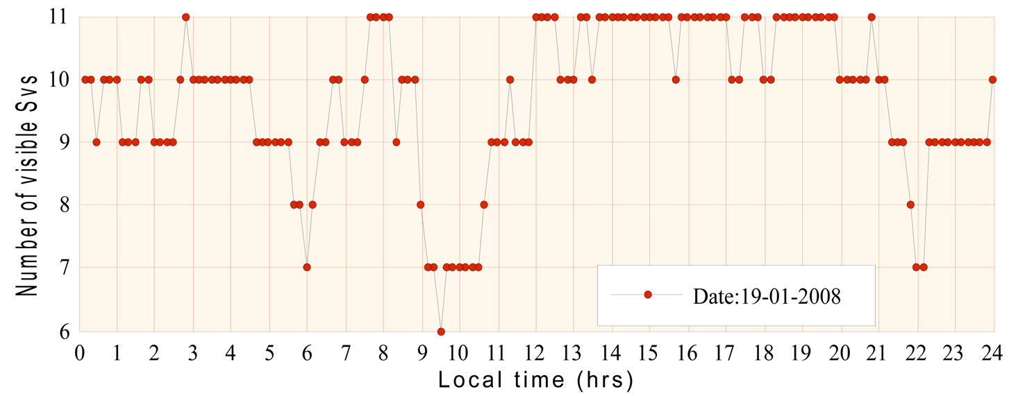
Figure 1. Local time Vs Number of visible satellites (SVs) on 19th January, 2008.
number of SVs (11) is visible mostly during 14-20 hrs.
2.2. Estimation of User Position Using Bancroft Algorithm
Bancroft algorithm (1985) estimates the preliminary coordinates for a GPS receiver. The algorithm requires ECEF coordinates of 4 or more SVs along with the values of their pseudoranges as input [8]. Figure 2 shows the variations in user position estimate with respect to local time. Variations in latitude are found to be negligible Figure 2(a). Variations in longitude are minimal Figure 2(b). Variations in height are relatively large Figure 2(c). From Figure 2(c) it can be observed that the algorithm gives unstable results for the starting of the day. Hence, standard deviation in height is 53.34 m in the first hour. However, over a period of 23 hours (1:00-24:00 hrs) standard deviation in height is reduced to 20.88 m. This value is in accordance with the value reported elsewhere [9]. Minimum, maximum, mean and standard deviation values of latitude, longitude and height are shown in Table 1. Standard deviations of latitude and longitude are minimal. Standard deviation of height is significant (53.34).
2.2.1 Estimation of User Position Using Kalman Filter
Kalman filter estimates the precise position of the receiver. The preliminary position estimated by the Bancroft algorithm is given as input to the Kalman filter along with the pseudoranges. Details on implementation of Kalman filter and other standard GPS related programs can be found elsewhere [9,10].
Figure 3 shows the variations in user position estimate with respect to local time. Latitude variations are negligible Figure 3(a). Minimum, maximum, mean and standard deviation of latitude, longitude and height are shown in Table 2. Variations in longitude are minimal Figure 3(b). Variations in height are relatively significant Figure 3(c). Standard deviation of latitude and longitude are negligible. However, standard deviation of height is relatively large (75.96).
2.3 Implementation of Filters before Estimating DOP
Various filters are available in literature to filter out some of the GPS errors while estimating pseudoranges before computing DOPs. DOPs are initially estimated without using any filter and are plotted with respect to local time for a period of 24 hours Figure 4. Subsequently, DOP values are estimated after incorporating Bayes filter. This filter is used to filter out GPS errors such as tropospheric error and receiver clock bias error from pseudoranges before estimating DOP values. Figure 5 indicates DOPs, plotted with respect to local time after implementing Bayes filter. Most of the time, Horizontal Dilution of Precision (HDOP) remained below 1. Vertical Dilution of Precision (VDOP) varies from 1.1 to
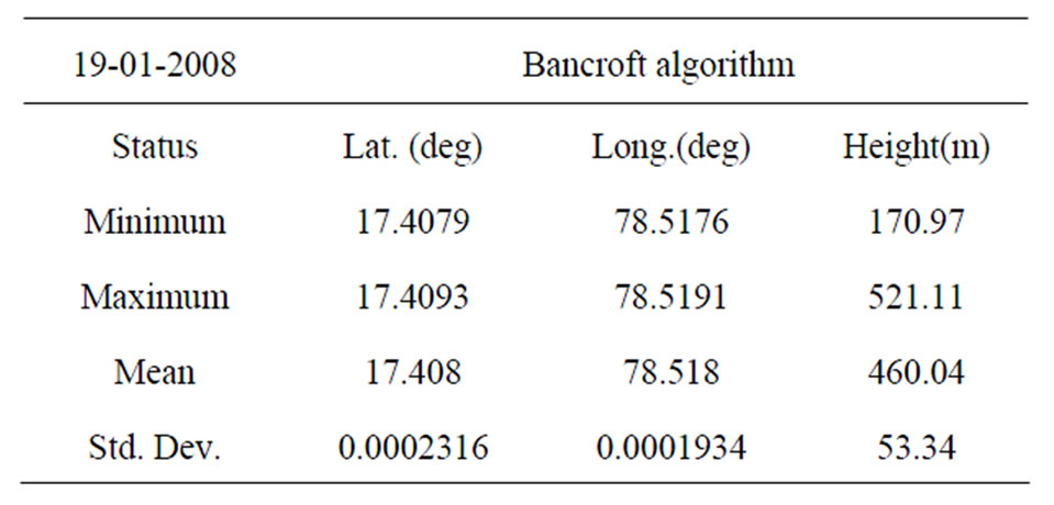
Table 1. User position estimated using Bancroft algorithm.
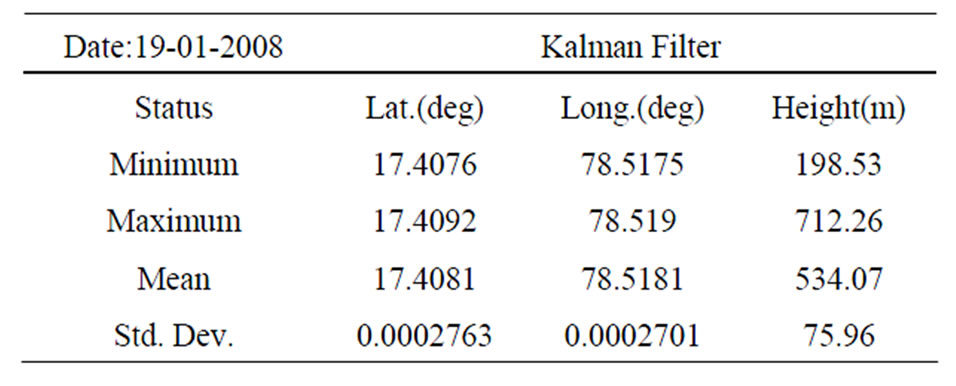
Table 2. Estimated user position using Kalman filter.
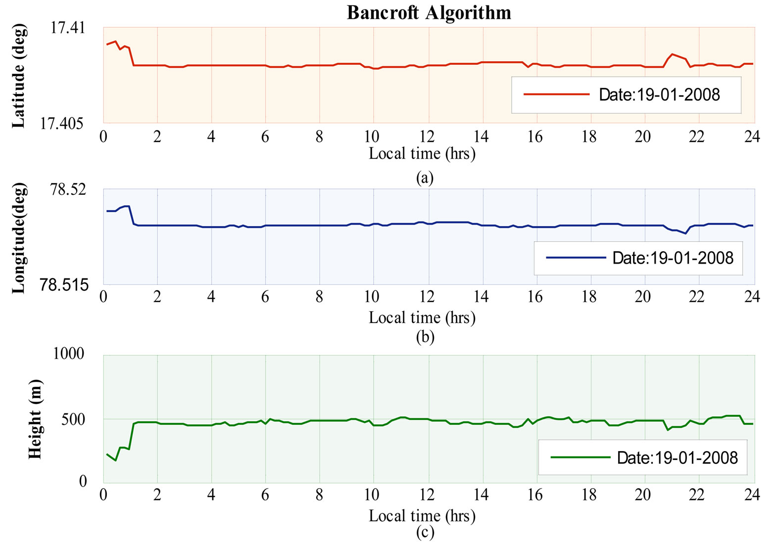
Figure 2. User (a) latitude (b) longitude and (c) height with respect to local time.
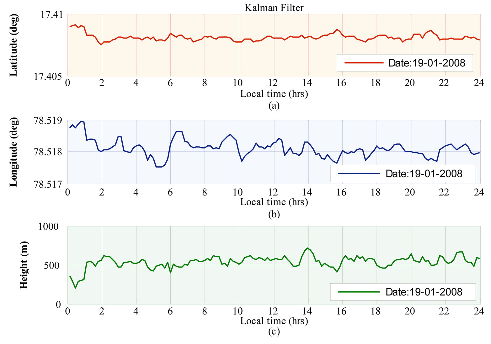
Figure 3. User latitude (a) longitude (b) and height (c) with respect to local time.
almost 3. Posi tional Dilution of Precision (PDOP) fluctuates from 1.32 to 3.59. Time Dilution of Precision (TDOP) variation is found between 0.57 and 2.62. Geometric Dilution of Precision (GDOP) varies from a minimum of 1.44 to a maximum of 4.45. Further, the DOPs are mathematically related as,
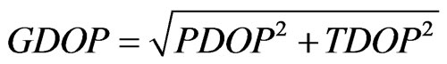 (1)
(1)
 (2)
(2)
The values of DOPs that are experimentally obtained satisfy these mathematical relations. Furthermore, the estimated values of HDOP, VDOP and PDOP are as reported elsewhere in open literature.
To see the effect of further filtering, Kalman filter is imposed on the pseudoranges corrected through Bayes filter. The results thus obtained are plotted in Figure 6. For most of the time, HDOP remains below 1. VDOP varies from 1.09 to 2.83. PDOP fluctuates from 1.32 to 3.11. TDOP variations are comparatively high and vary from 1.82 to 7.08. GDOP varies from a minimum of 2.26 to a maximum of 7.73. The values of DOPs satisfy their mathematical relations (Equations (1) and (2)). Further, the estimated values of HDOP, VDOP and PDOP are cross-validated with the values reported in open literature. As stated, HDOP remains less than one almost at all times; VDOP is usually higher than HDOP. PDOP will be generally lower than 3 in lower latitude regions. Standard deviation of VDOP is supposed to be twice than that of HDOP [11].
For comparative analysis minimum, maximum, mean and standard deviation of DOPs are estimated for the three cases and are tabulated in Table 3.
Comparing three cases for PDOP, it is observed that PDOP (max) is least (3.09) when no filter is used, it is highest (3.59) when only Bayes filter is used and it is medium (3.11) when Kalman filter is incorporated. Kalman filter provides more precise position than Bancroft algorithm which uses Bayes filter. However, implementation of Kalman filter is complicated and highly time consuming compared to Bayes filter. Further, when the user position estimated by the Kalman filter is utilised along with the positions of visible SVs, then the DOP values are found to be similar to that of due to Bayes filter (kom.aau.dk/~borre/matlab/–2k). However, when the DOP values are estimated using the covariance matrix provided by the Kalman filter, significant difference is found when compared to the estimations due to the previous methods Table 3.
3. Augmentation of GPS with Pseudolites
There are various applications of augmented GPS such as mining, vehicle tracking and aircraft landing etc. However, the advances in pseudolite technology enable them to play key role in aircraft landing [12]. In this paper, a typical LAAS scenario is considered and augmented with simulated pseudolites’ positions to investigate their effect on DOPs.
3.1. Investigation on the Effects of Pseudolites’ Placement on DOPs
We have considered three configurations of the pseudolites placed in different ways to investigate their effect on DOPs Figure 7.
It is assumed that the aircraft is equipped with two antennas on top and one antenna in the bottom [13]. One top antenna receives VHF signals from DGPS station and the other top antenna receives signals from GPS. The bottom antenna receives pseudolite signals. Further, it is assumed that the aircraft is approaching (making an angle of 3˚) towards the runway touchdown point through the glide path [14]. This angle is called as glide slope. Further, it is assumed that the horizontal coverage distance is 20 nm (37 km). This leads to a maximum altitude of 1.94 km just before aircraft enters the glide path. Also, it is considered that APL3 is posi tioned at 6.5 km from the touchdown point in the direction of runway and APL1 and APL2 are placed on either side of the run way at a disoptance of 6.5 km from the touchdown point [15].
For the purpose of analysis, mean value of the receiver position is considered Table 1 and its altitude is scaled to 1.94 km (= 2461 m (MSL)) to make it work like an airborne stationary receiver over Hyderabad Table 4. Subsequently, GPS is augmented by simulated coordinates of airport pseudolites (APLs) by selecting different number of APLs each time. DOPs are estimated using‘all-inview’ SVs. Table 4 shows the simulated geodetic
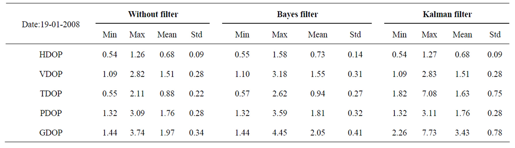
Table 3. Minimum, maximum, mean and standard deviation of DOPs before and after implementing filters.
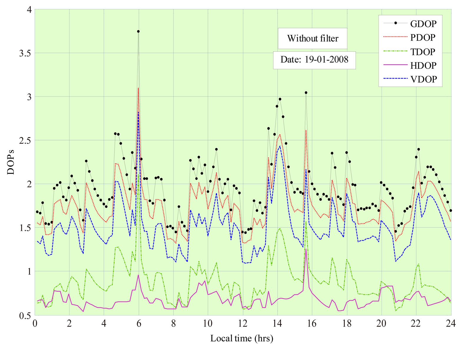
Figure 4. DOPs with respect to local time without filters.
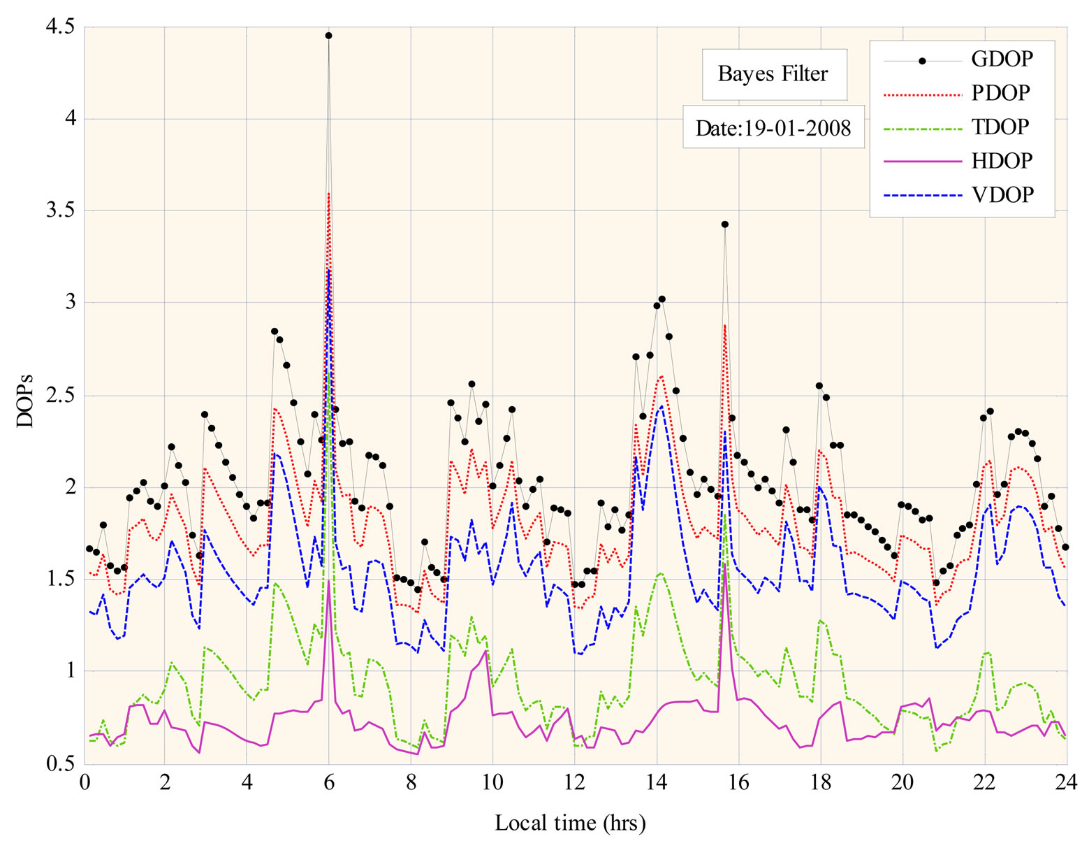
Figure 5. DOPs with respect to local time after implementation of Bayes filter.
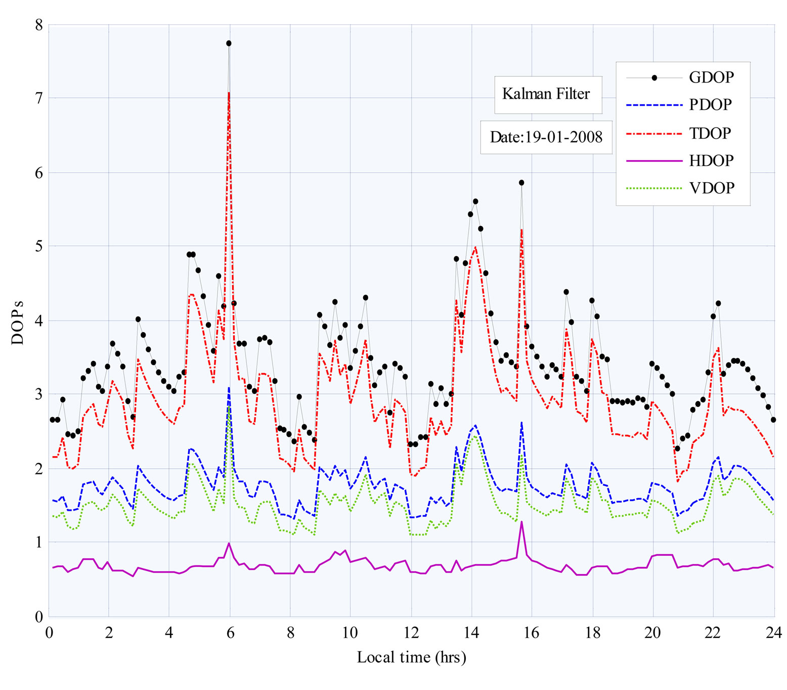
Figure 6. DOPs with respect to local time after implementation of Kalman filter.

Figure 7. A typical LAAS scenario with APLs.
coordinates of the APLs and the user with scaled height.
With and without augmentation with APLs, variations in GDOP, PDOP, VDOP, HDOP and TDOP with respect to time are estimated and results are shown in Figures 8-12.
Comparing all the figures, it can be observed that GDOP, PDOP, VDOP, HDOP and TDOP values are the highest when only GPS is available. Due to the presence of APLs good improvement is found in all the DOPs. As the number of APLs is increased, DOP values are found to be decreasing. The least DOP values are obtained when two APLs (APL1 and APL2) are used. The DOP values due to APL1 as well as APL3 are found to be similar.
Table 5 shows minimum, maximum and standard deviation of DOPs with and without APLs. From Table 5 it can be observed that the maximum value of VDOP remains below 3 and of HDOP remains below 1.27 for all the configurations.
The maximum PDOP has crossed 3 when no augmentation is there. It is around 2 when augmentation exists. TDOP became half due to augmentation. GDOP is nearly 4 without augmentation and comes down to approximately 2 due to augmentation. The standard deviation of all the DOPs is higher for standalone GPS compared to that of augmented GPS. For all DOPs, standard deviation is remaining almost constant for all the augmented configurations.
4. Conclusions
For GPS based navigation systems, improvement in DOP can be achieved using pseudolites. In this paper, a typical LAAS scenario is considered and the effect of pseudolite placement on DOP enhancement is investigated. For this purpose, pseudolites are positioned in different locations and DOP values are estimated. It is found that the locations of the APLs and also the number of APLs affect the DOPs. DOPs with two APLs (APL1 and APL2) are found to be the best. Whether the APL is positioned before the runway or beside the runway no significant difference is found in DOP values. For all the configurations, maximum value of VDOP remained below 3 and that of HDOP remained below 1.27. Due to only GPS, PDOP (max) crossed 3 and it became approximately 2 due to augmentation. TDOP became half due to augmentation. GDOP was found to be nearly 4 due to GPS alone and came down to approximately 2 due to augmentation with two APLs. Though Kalman filter provides better accuracy, it is complicated and time con-

Table 4. Simulated coordinates of the APLs and the user.
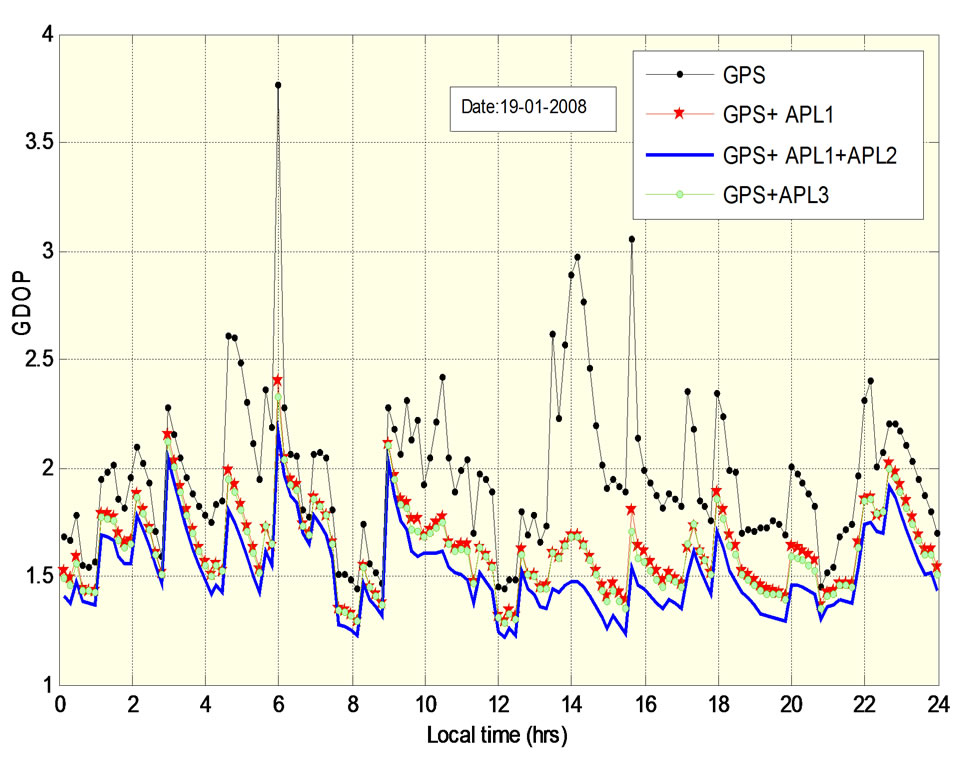
Figure 8. GDOP variations with and without APLs.
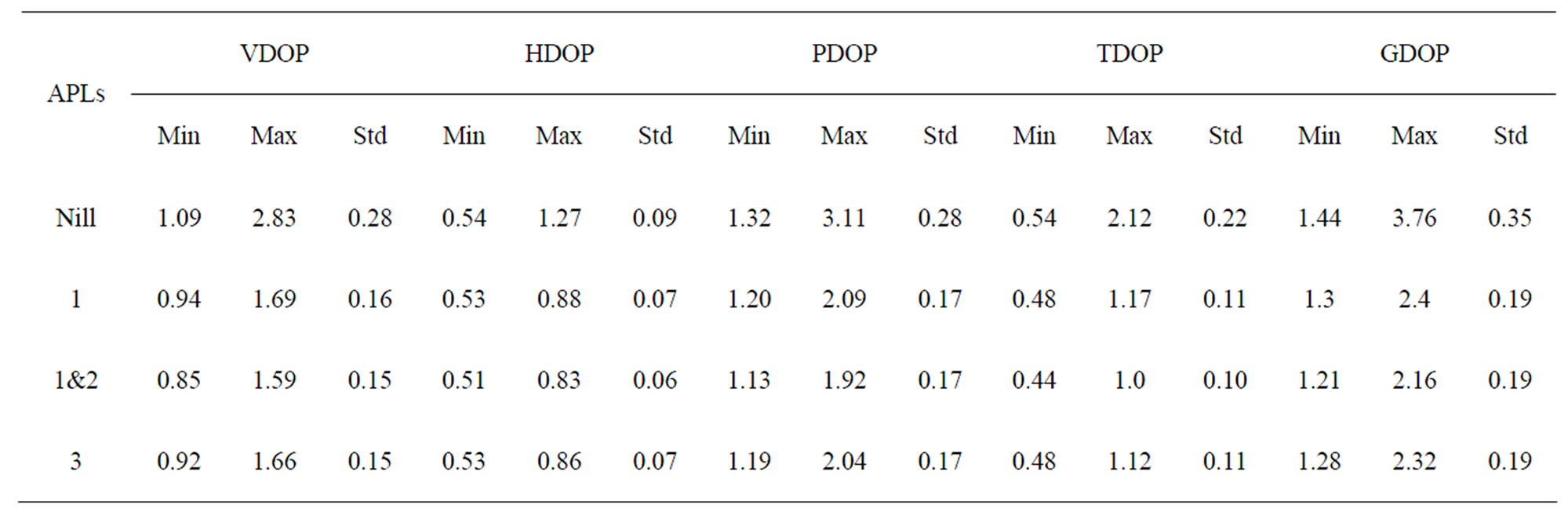
Table 5. Minimum, maximum and standard deviation of DOPs with and without APLs.
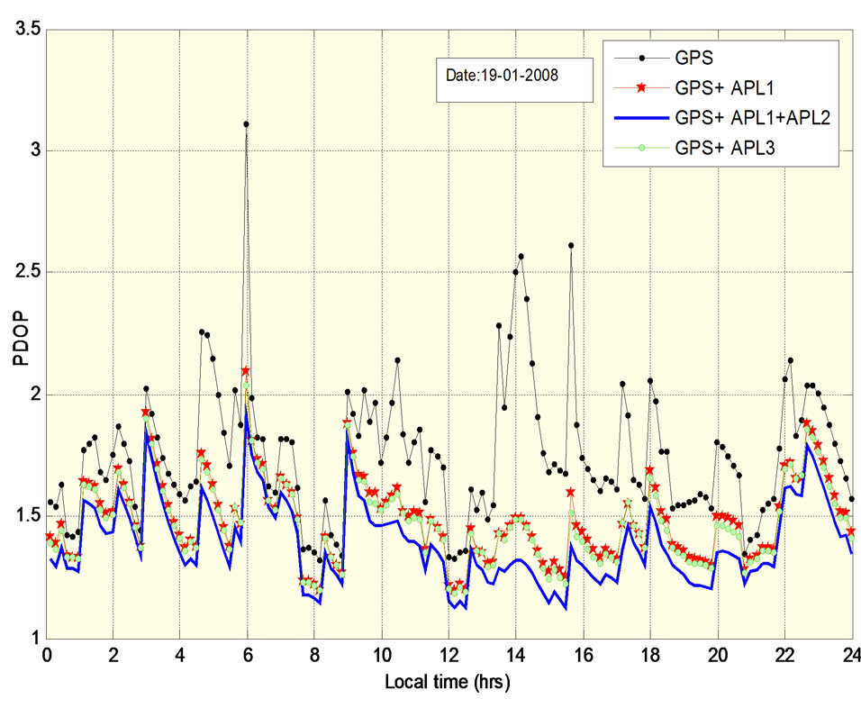
Figure 9. PDOP variations with and without APLs.
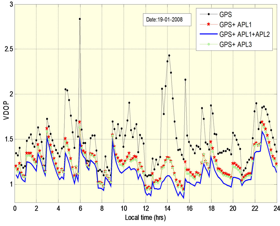
Figure 10. VDOP variations with and without APLs.

Figure 11. HDOP variations with and without APLs.
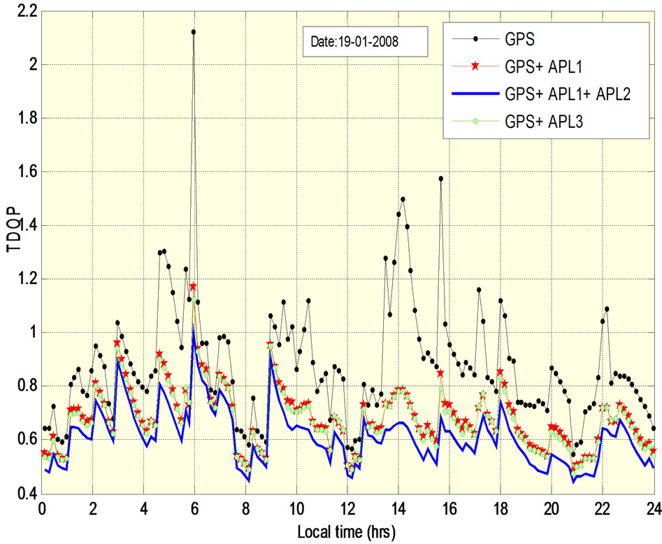
Figure 12. TDOP variations with and without APLs.
suming compared to that of Bayes filter.
5. Acknowledgements
The above work has been carried out under the project entitled “Investigation of Atmospheric Effects on Future Ground Based Augmentation for GPS System” sponsored by Department of Science and Technology, New Delhi, India, vide sanction letter No: SR/S4/AS:53/2010, dated: 12th July 2010.
REFERENCES
- B. D. Elrod and A. J. Van Dierendonck, “Pseudolites,” In: B. W. Parkinson and J. J. Spilker, Ed., Global Positioning System: Theory and Applications (Vol. 2), American Institute of Astronautics, Washington D.C., 1996, pp. 51- 79.
- R. L. Harrington and J. T. Dolloff, “The Inverted Range: GPS User Test Facility,” IEEE PLANS’76, San Diego, California, 1-2 November 1976, pp. 204-211.
- E. Lemaster and S. Rock, “Mars Exploration Using Self-Calibrating Pseudolite Arrays,” 12th International Technical Meeting of the Satellite Division of the Institute of Navigation GPS-99, Nashville, Tennessee, 14-17 September 1999, pp. 1549-1558.
- “FAA Approves 1st U.S. Ground Based Augmentation System,” U.S. Federal Aviation Administration Washington Headquarters Press Release, 21 September, 2009.
- K. Zimmerman, “Experiments in the Use of the Global Positioning System for Space Vehicle Rendezvous,” Ph.D. Thesis, Stanford University, California, 1996.
- “Minimum Operational Performance Standards for GPS Local Area Augmentation System Airborne Equipment,” Washington D.C., RTCA SC-159, WG-4, DO-253C, 16 December, 2008.
- S. Bancroft, “An Algebraic Solution of the GPS Equations,” IEEE Transactions on Aerospace & Electronics Systems, Vol. 27, No. 6, 1985, pp. 56-59.
- K. Borre, “GPS MATLAB Tools at Aalborg University by Kai Borre,” May 2010. http://kom.aau.dk/~borre/matlab/-2k
- K. Borre and G. Strang, “Linear Algebra Geodesy and GPS,” Wellesley-Cambridge Press, USA, 1997.
- R. G. Brown and P. Y. C. Hwang, “GPS Failure Detection by Autonomous Means Within the Cockpit,” Proceedings of the Annual Meeting of the Institute of Navigation, Seattle, WA, 24-26 June 1986, pp. 5-12.
- P. Misra and P. Enge, “Global Positioning System-Signals, Measurements and Performance,” Ganga-Jamuna Press, Lincoln, Massachusetts, USA, 2001.
- C. G. Bartone, and S. Kiran, “Flight Test Results of an Integrated Wideband Airport Pseudolite for the Local Area Augmentation System,” ION-GPS, Salt Lake City, Utah, 2000.
- C. E. Cohen, B. S. Pervan, H. S. Cobb, D. G. Lawrence, J. D. Powell and B. W. Parkinson, “Real-Time Cycle Ambiguity Resolution Using a Pseudolite for Precision Landing of Aircraft with GPS,” DSNS ’93, Amsterdam, The Netherlands, 30 March-2 April 1993, pp. 171-178.
- S. Fukushima, T. Yoshihara and S. Suga, “Evaluation of a Tropospheric Correction Model for Airport Pseudolite,” 17th International Technical Meeting of the Satellite Division of the Institute of Navigation, Long Beach, CA, 21-24 September 2004, pp. 2283-2288.
- W. B. Parkinson and J. J. Spilker, “Global Positioning System: Theory and Applications: Vol. 1 and 2,” American Institute of Aeronautics and Astronautics, Inc, Washington, 1996.