Journal of Geographic Information System
Vol. 4 No. 6 (2012) , Article ID: 26318 , 11 pages DOI:10.4236/jgis.2012.46055
Proposal for the Introduction of the Spatial Perspective in the Application of Global Sensitivity Analysis
1Faculty of Earth Sciences and Space, Autonomous University of Sinaloa, Culiacan, Mexico
2Department of Geography, University of Alcalá, Alcalá de Henares, Spain
Email: wenses@uas.edu.mx, montserrat.gomez@uah.es, joaquin.bosque@uah.es
Received October 2, 2012; revised November 3, 2012; accepted December 5, 2012
Keywords: Sensitivity Analysis; Geographical Information System; Multi-Criteria Evaluation; Simulation of Urban Growth; Madrid Region (Spain)
ABSTRACT
In any model, Sensitivity Analysis (SA) is a fundamental process to improve the robustness and credibility of the results, as part of validation procedure. Generally, SA determined how the variation in the model output can be apportioned to different sources of variations, and how the given model depends upon the information fed into it. Many complex techniques of SA have been developed within the field of numerical modeling; however, they have limited applications for spatial models, as they do not consider variations in the spatial distributions of the variables included. In this research, a variation in the implementation of a Global Sensitivity Analysis (E-FAST) is proposed in order to include the spatial level. For this purpose the conventional tools available in a raster Geographical Information System (GIS) are used. The procedure has been tested in a simulation of urban growth for the Madrid Region (Spain) based on Multi-Criteria Evaluation (MCE) techniques. The results suggest that the inclusion of the spatial perspective in the application of the SA is necessary, because it can modify the factors that have a decisive influence on the results.
1. Introduction
With increasing frequency, new methodologies are being applied during the preparation stage of land use planning proposals in order to construct spatial simulations of a series of possible alternatives for future land use and thus facilitate more informed planning decisions. These methodologies allow the spatial combination of different economic, social, environmental and terrain criteria; weighted according to the level of importance, they have been assigned by expert groups, decision makers or social agents. Consequently, planning is both more comprehensive and participative. In the context of land use analysis, the Multi-Criteria Evaluation (MCE) method is one of the most frequently used approaches for simulateing desirable or optimal future land allocation scenarios. However, the results of these simulations sometimes have not produce enough confidence because the subjectivity of the weighting factors process or the fact that we cannot verify the outputs of the model with real data, because they are simulating only possible images of the future ([1] Barredo Cano and Gómez Delgado, 2008). However, any model should be validated in order to improve its robustness and acceptability ([2] Verburg et al., 2004; [3] Gómez Delgado and Bosque Sendra, 2009). If we are modelling a future system state, we should carry out a partial validation, for example, exploring the stability of model outputs ([4] Pagelow and Camacho Olmedo, 2008: 29).
One possibility for assessing a certain level of confidence on the results of these spatial simulation models is provided by Sensitivity Analysis (SA) ([2] Verburg et al., 2004; [1] Barredo Cano and Gómez Delgado, 2008; [5] Qureshi et al., 1999; [6] Chu-Agor, et al., 2011). This type of analysis could determine the stability or robustness of the model results by studying to what extent the results are affected by small changes to the input parameters. It can be useful to improve individuating which factors need to be measured accurately in the model, in order to achieve enough precision ([7] Crosetto et al., 2000: 73). Furthermore, it can help to simplify the originnal model and reduce computational demand, giving important insights for the optimization of GIS data acquisition resources ([7] Crosetto et al., 2000; [8] Saltelli et al., 2000; [9] Saltelli et al., 2008).
In many studies we can find the use of SA as synonyms of Uncertainty Analysis (UA). We avoid using the term uncertainties because we think it takes another sense when we talk about spatial data. In that context, the UA is about studying any possible (and not very well known) errors affecting the initial data to find out how they modify the results ([3] Gómez Delgado and Bosque Sendra, 2009). The SA procedure is based on small changes in the initial range of the variables that not always could be considered properly as errors. The SA rather sought to determine the influence of each factor in the variance of the model results.
Out of the different methods employed to carry out SA (Screening, Local and Global), the most frequently used in a variety of fields where numerical models are considered (economics, engineering, chemistry ...) are global methods (Sobol’, Fast, E-Fast), since these make possible simultaneous analysis of all possible interactions between input variables and model output results ([8] Saltelli et al., 2000). In addition, it can be applied to MultiCritera Evaluation based models, partitioning the variance of result model into model input factors and weights ([10] Saltelli et al., 1999).
However, in studies which have applied a spatial MCE approach (usually based on a GIS), the use of SA as part of the validation process has been scarce or limited, as demonstrated in the literature reviews conducted by [5] Qureshi et al., (1999) and [11] Gómez Delgado and Bosque Sendra (2004). Some changed the order of preference assigned to each criterion or objective ([5] Qureshi et al., 1999; [12] Pettit, 2002; [13] Chang et al., 2008), whilst others introduced variations in the values assigned to model parameters (weightings, distance metrics, etc.) ([14] Jankowski, 1995; [15] Baja et al., 2007) or applied different aggregation methods in order to convert suitability maps (based on pixels) into environmental zoning maps (based on pixel groups) ([16] Geneletti and van Duren, 2008).
Global Sensitivity Analyses are essentially based on the definition of a Probability Distribution Function (PDF) for each model input variable, from which a sample is extracted. The model is then run a significant number of times, generally applying a Monte Carlo simulation ([8] Saltelli et al., 2000). This procedure becomes more difficult when spatial or temporal input variables are considered ([17] Lilburne and Tarantola, 2009), because we should take into account variations in each part of the space or time considered.
Nevertheless, these methods have been used for many different spatial models ([7] Crosetto et al., 2000; [18] Crosetto and Tarantola, 2001; [19] Gómez Delgado and Tarantola, 2006; [20] Wagener and Kollat, 2007; [21] Tang et al., 2007; [17] Lilburne and Tarantola, 2009; [22] Varella et al., 2010; [7] Chu-Agor et al., 2011). However, the spatial variability of the factors used in the model is not considered. In addition, on a GIS-based MCE approach, when numerical SA methods are applied, only variations in PDF of the weights are introduced, omitting the factors from the analysis1.
In this context, Lilburne and Tarantola (2009) [17] conducted an exhaustive review of numerical SA techniques applied to spatial models and found a series of deficiencies in such applications. In particular, their review highlighted the importance of basing SA on variations in weighting distribution and also in the distribution of input variables. It is also very important to take into consideration the entire spatial structure, in order to analyze the importance of each spatial input, instead of reducing the spatially variable inputs to a single scalar value. In their research the authors implemented SA to evaluate a groundwater contaminant model caused by agricultural activity in New Zealand (Test Example 1), using an adapted version of the Sobol’ method in order to determine which of the variables were most significant or had a decisive influence on the results of the model. The results show that the resolution of the input maps, as well as the magnitude of variability of each input, can determine the outputs of the model. However, though the model is a weighted composite index, the authors do not consider the effect of the weights.
The aim of this paper is to carry out a partial validation of a model for simulating future urban growth in the Madrid Region using GIS-based MCE techniques, through a sensitivity analysis in order to determine the stability/ robustness of the model results. Our main objective is to develop a procedure to apply a global SA method considering the spatial characteristics of the model, avoiding the reduction of the spatially variable inputs to a single scalar value. This alternative procedure takes into account the variables (called factors in MCE) and weights attached. This proposed procedure is easy and intuitive to apply, using the tools available within a raster-based GIS environment. SA was conducted with the Extended Fourier Amplitude Sensitivity (E-FAST) method, using the SimLab2 software.
2. Study Area, Model of Urban Growth and Data
The SA was applied on the results of a model for simulating and allocating new urban land in the Madrid Region. This region was selected because the impacts of the rapid housing development process registered in the last 10 - 15 years (Figure 1). The main consequence of it has been land occupation based on dispersed housing estates: between 1990 and 2000, approximately 50,000 Ha disappeared under artificial surfaces ([23] EEA, 2006; [24] Plata Rocha et al., 2009).
We present a summary of the model and the main
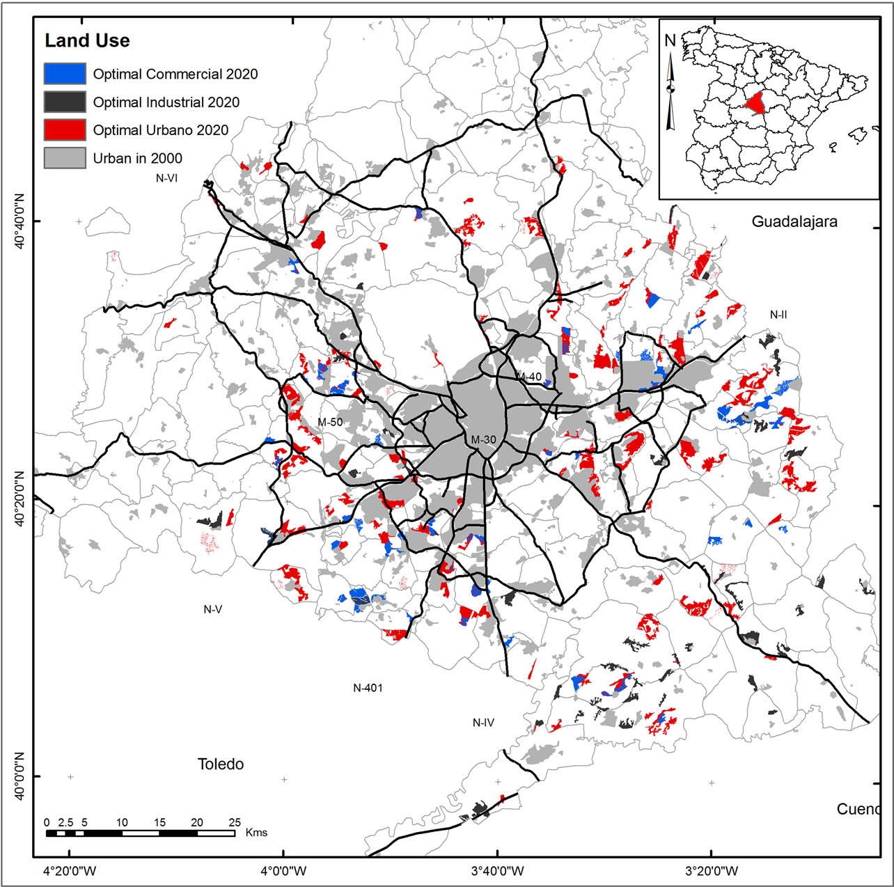
Figure 1. Results of the optimal allocation model for residential, industrial and commercial use in the Madrid region (year 2020).
results. In [25] Plata Rocha et al., 2010 it is possible to find a complete description of the scenario analyzed here. Further description of this scenario of future urban growth (innovation and sustainability) and two more models developed for 2020 (business as usual scenario and crisis scenario) in [26] Plata Rocha et al., 2011.
In order to implement the model, the land occupation scenario for the year 2000 was taken as a basis. An optimal residential, industrial and commercial land use allocation procedure was carried out for the year 2020, considering up to 16 variables related to environmental, economic and social aspects, weighted (via the pairwise comparison matrix of the Analytic Hierarchy Process) according to their level of importance for this purpose (Table 1).
A Weighted Linear Combination (Equation (1)) MultiCriteria Evaluation method was employed to produce the suitability maps (residential, commercial and industrial):
 (1)
(1)
where: MS is the map representing each pixel’s level of suitability for development; and wi is the weight of each

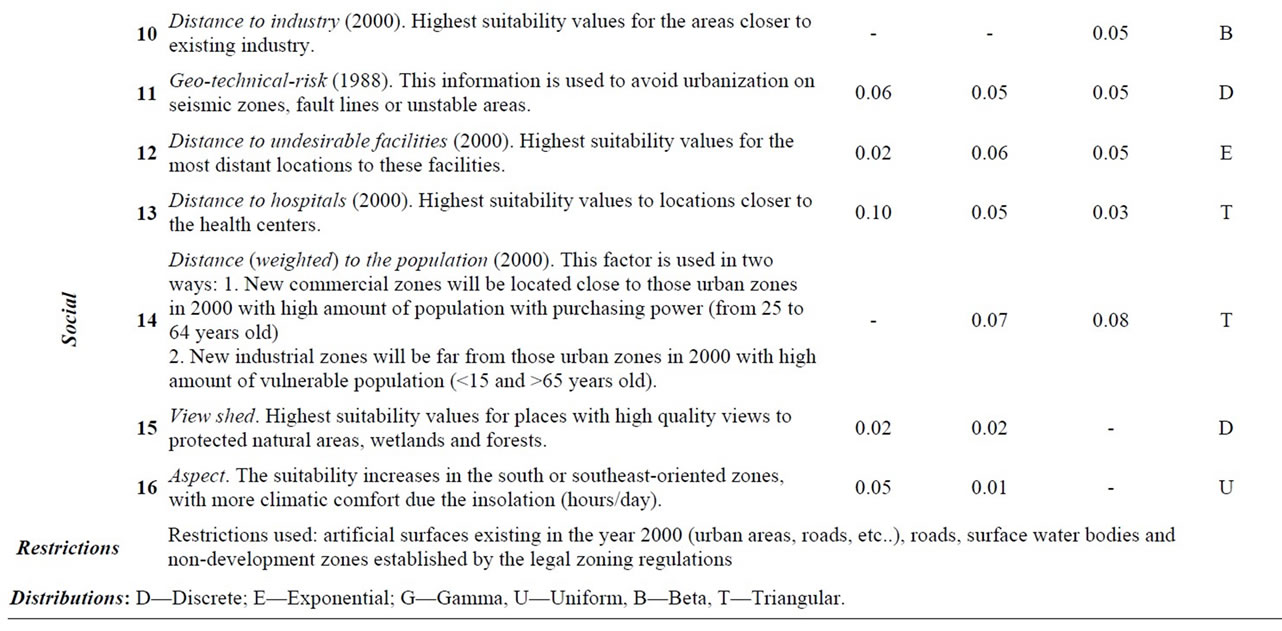
Table 1. Description, type of distribution and weight of the variables (factors in MCE context) used in the urban growth model for year 2020 in the Madrid Region (Plata Rocha et al., 2010, Plata Rocha et al., 2011).
variable (factor) Xi. MR is the map representing the restricted areas to the activities specified in the model.
The final maps of the most suitable parcels for each land use were generated from the suitability maps. The demand was determined externally, using a Systems Dynamics model and different socio-economic and demographic variables (see [27] Aguilera Benavente et al., 2009 for a detailed description of this procedure).
Lastly, using the maps of suitable parcels for residential, commercial and industrial use, multi-objective land allocation was applied (IDRISI; MOLA module) in order to solve possible allocation conflicts between the three uses. As a result, an urban growth allocation model for 2020 was obtained (Figure 1).
3. Methodology
The SA procedure was conducted in two methodological stages, illustrated in Figure 2. In the first stage (3.1), the SA was performed applying the E-FAST method. In the second (3.2), a spatial-explicit E-FAST was conducted.
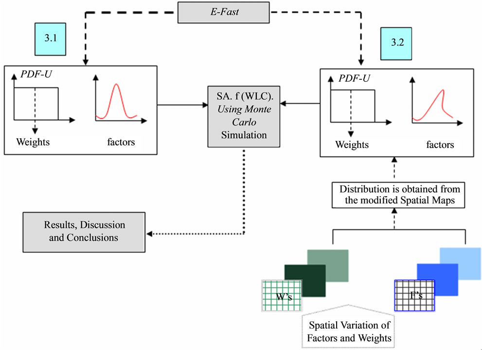
Figure 2. Methodological framework of the SA. The analysis 3.1 is based on the E-FAST method. The 3.2 is the proposed spatial E-FAST.
3.1. Extended Fourier Amplitude Sensitivity Test (E-FAST)
This technique was developed by [28] Saltelli et al., (1999) from the theoretical and mathematical bases of the FAST method proposed by [29] Cukier et al. (1975). It is considered to belong to the group of techniques based on variance estimation. In order to obtain first order and total effect sensitivity indices through application of this technique, a Monte Carlo simulation sample is used considering k independent input factors and a number N of samples.
For a given factor, the sensitivity index represents the fractional contribution to the variance of the model output which is due to this factor. In order to calculate the sensitivity indices, the total variance V of the model output is apportioned to all the input factors Xi as follows:
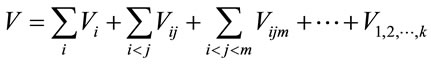 (2)
(2)
where: 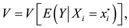
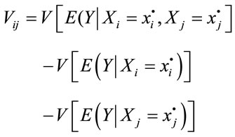
And so on. In the formulas above, Y denotes the output variables, Xi indicates an input factor, 
marks the expectation of Y conditional on Xi, and V shows conditional variance.
The sensitivity index Si for the factor Xi is defined as:
 (3)
(3)
It represents the part of variance of Y explained by Xi. The most important contribution of E-FAST is that for each Xi it provides a first order sensitivity estimate Si and a total sensitivity index estimate STi. It is possible to observe the difference between the impact of factor Xi on Y alone, measured by Si and the total impact of factor Xi due to interactions with other factors in model Y, measured by STi.
The E-FAST and other techniques are implemented on SimLab Software, used to conduct the SA as follows:
1) The frequency distribution of factors was determined (last column of Table 1) using the tools of the GIS to obtain the frequency histogram of cell values of each factor. In the case of weightings, uniform distribution was assigned with a ±25% variation with respect to their nominal values;
2) A sample was generated from the different model factors (variables and their corresponding weights) taking into account each frequency distribution and the model was then run a substantial number of times (4941 repetitions in this case);
3) Finally, the values obtained for the sensitivity indices of the model input factors were analyzed.
3.2. Proposal of a Spatial E-FAST Method
The previous methodology presents the disadvantage that is based on the PDF of the variables and weights included in the model, but not taking into account the spatial distribution of them. Therefore, we proposed a procedure to include the spatial variability of the all factors in order to construct an alternative PDF of them from which we extract the samples to run the model, using the tools available in a conventional raster GIS (Idrisi).
The proposed methodology is based on the random introduction of a certain percentage of variation in the suitability values obtained for the spatial variables and in the weights at pixel level (originally a nominal value), as shown in diagram in Figure 3. The interval of the variation used was ±25%. This interval is similar to that used in other studies ([18] Crosetto, and Tarantola, 2001; [19] Gómez Delgado y Tarantola, 2006). The sensitivity analysis must be done through small variations in the original conditions of the model because if this amount is increased, we could change completely the original model.
The procedure for the variables (MCE factors) is illustrated in the left part of the figure. First of all, a new raster map with random values from 0.75 to 1.25 for each pixel is generated. This map and one of the factors maps included in the model (with the suitability value related with this variable for each pixel) are overlaid with a multiplying operation and the final factor map, with ±25% interval of variation respect to the original value, is obtained. This procedure ensures that each pixel of the raster map for each variable included in the model has a variation of ±25% of the original suitability value. Note that this procedure avoids a uniformed distribution of spatial uncertainty.
The right part of Figure 3 represents the procedure for the weights. Now, the first raster map is generated with random values between 0.75 and 1.25. Next, this image is multiplied for the weight nominal value to obtain an image with a spatial variation of ±25% of the original weight. For instance, the variable (factor map) land use has a weight of 0.14. Then a random value between 0.105 (−25%) and 0.175 (+25%) will be assigned to each pixel of the land use factor map. We consider that, in a variety of MCE models, a factor is weighted differently depending on the sub-area. In fact, the land use factor was modeled on this way ([26] Plata Rocha et al, 2011). So it seems appropriate to include an assessment of the impact of this possible process in the overall variance of model output.
Then, the implementation of a random variation at pixel level in the factors and weights guarantees that any pixel had the same probability to change their values within the ranges proposed.
These two operations were performed for the 13 variables (factor maps) and for the 13 weights attached to each factor, obtaining 26 new raster images. As mentioned earlier, E-FAST method is based on the definition of a Probability Distribution Function (PDF) for each model input variable, from which a sample is extracted. Thus, the procedure was as follows:
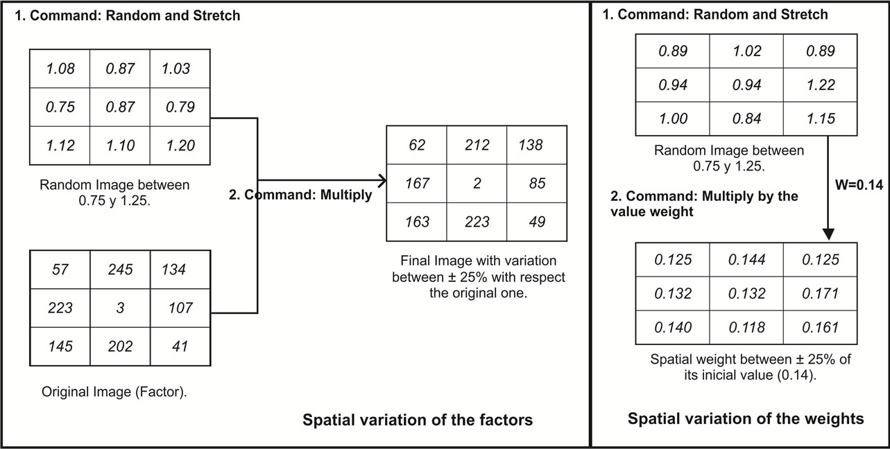
Figure 3. Process to obtain the variation on the spatial factors (left) and weights (right).
1) First of all, we can obtain the different PDF from these modified maps, where the variation of the original value was made for each pixel of the map (see two examples in Figure 4);
2) Then, we can consider that the samples extracted from these PDFs take into account the spatial level. In the other hand, variations in the PDF of all factors of the model (variables and weights attached) are introduced, following the argument proposed by [17] Lilburne and Tarantola (2009);
3) Lastly, with these new inputs, the SA procedure was applied as that one described in Section 3.1 in the point II and III.
Finally, in order to compare and analyze the results obtained from the E-FAST method and the Spatial E-FAST method, the sensitivity indices Si and STi were employed.
4. Results
4.1. Results of the E-FAST Method
According to the results obtained for conventional application of the E-FAST method, shown in Table 2, the factor assigned the highest proportion of variability in results was land use (0.24 and 0.17 in the case of residential and commercial zones, and up to 0.48 for industrial zones). In addition, it can be seen that a further 4 factors presented a certain measure of variability, including distance to urban centers, in the residential land use model (0.14) and the commercial land use model (0.15), distance to commercial centers in the commercial land use model (0.15), soil type in the industrial land use model (0.13), and Geo-technical-risk in the residential land use model (0.09).
Finally, the results obtained were typical of that found for almost all the models, that is, only three or four factors were found to have a significant influence on the results. However, what is unusual in this case is that the proportion represented by the sum of the most important factors was relatively low compared to what is typically found in other models ([30] Crosetto et al., 2001; [31] Crosetto et al., 2002; [19] Gómez Delgado and Tarantola, 2006). Since much of the variance in results was not reflected, it would be inappropriate, for example, to use this information in order to simplify the model. The results show that all of the factors are necessary for the correct application of the model.
4.2. Results of the Spatial E-FAST Method
As described in Section 3.2, the E-FAST method was once again applied, taking into account the spatial variance of the model factors.
Results show that at least 9 variables presented a considerable amount of variability in the model (Table 3). The results demonstrate that once variations had been introduced, both for variables and weights, a further 3 significant factors were obtained in addition to those identified in the first analysis (distance to surface water bodies, distance to natural protected areas and distance to roads). Factors like distance to hospitals and aspect, with low influence in the first procedure, disappear in this new E-FAST application.
Another interesting result is the reduction of the importance of the land use factor. When the spatial level is taken into account, this factor keeps its importance only for the industrial land use model. Distance to urban centers takes now the first place in the residential land use model.
In addition, other two main differences were found. In one hand, the sum of the most important factors has increased. This opens the possibility to erase from the model the more insignificant factors, because there are enough factors that are reflecting the variance of the model. In the other hand, the difference between the first order and total effect indices (Si and STi) indicated that there is an interaction among the inputs, although the difference between these is not significant (<0.2). Note that in the first procedure the results for both indices were the same for all the factors.
Finally, the results of both procedures confirm that the weights attached to the variables are robust and the introduction of small variations does not influence the variation of the results of the model.
5. Conclusions
Although many numerical techniques currently exist to carry out a SA of different types of models, these procedures lack the spatial perspective. This article proposes an alternative approach to redress this limitation. In our study, it was observed that the SA only identified a maximum of 5 significant factors when using the PDF of the parameters and when the only changes introduced corresponded to variations in the distribution of weights (Table 2). However, when a SA was performed considering the PDF of factors with pixel-level variations, other influential factors were identified.
We consider that, to a certain extent, the use of this kind of SA redresses the deficiencies presented by other methods when applied to spatial models. In addition, this spatial perspective is easy to perform with the basic tools available in a conventional GIS. It is very important to take into account this question in order to encourage the realization of the validation procedure of a model, which it is not frequently carried out because of the effort and time that it usually takes.
We can confirm that, based on the application of the two SA methodologies described; the most important, influential and significant factors regarding the model for
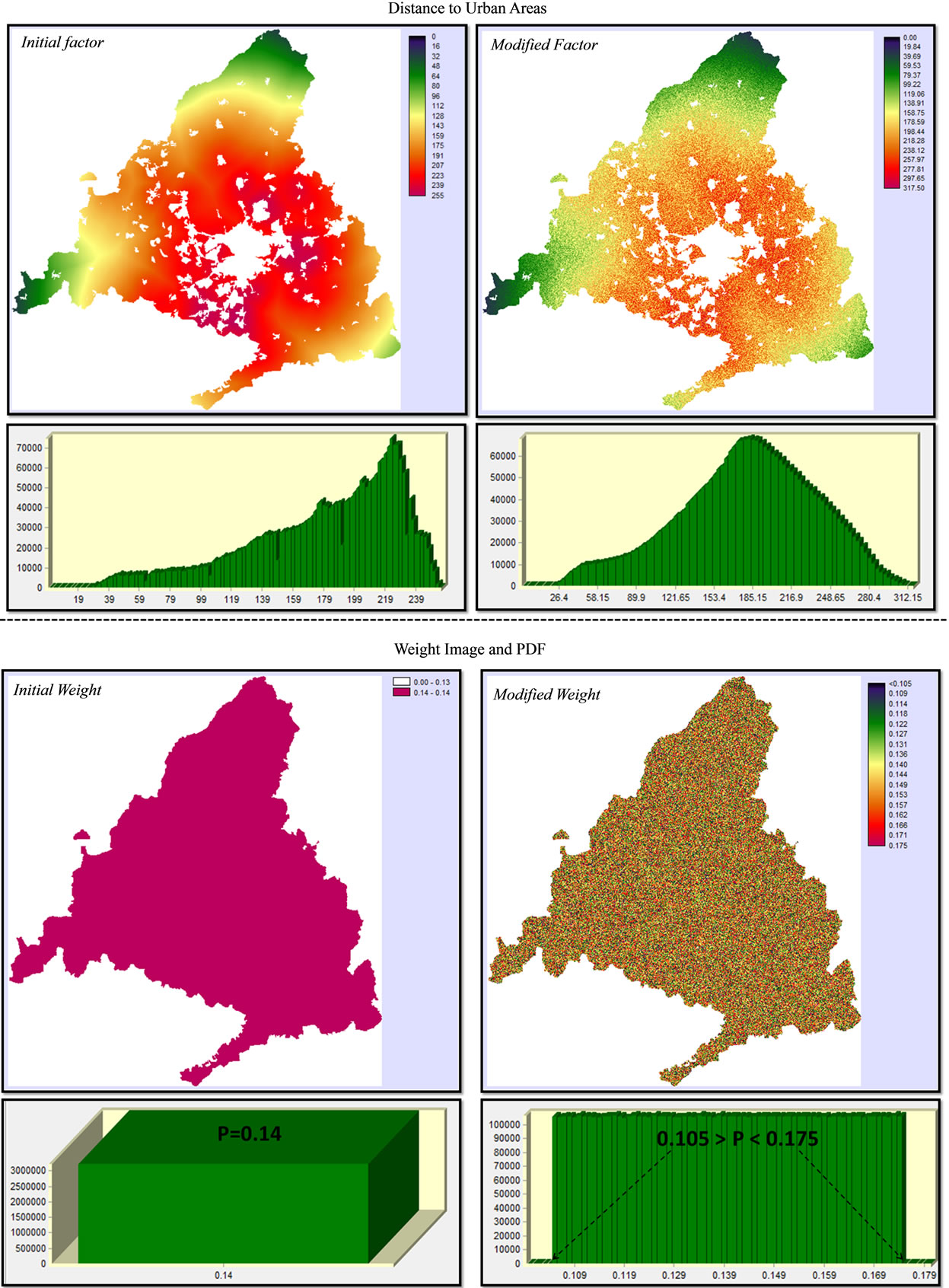
Figure 4. Original spatial version and modified spatial version of distance to urban areas factor and its weight.
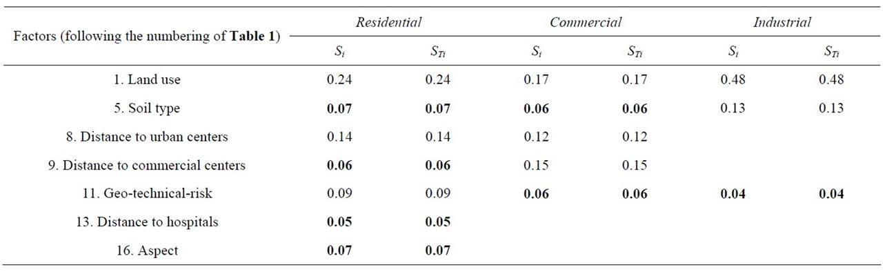
Table 2. Most significant factors in the SA, after introducing variations of ±25% in the weights.
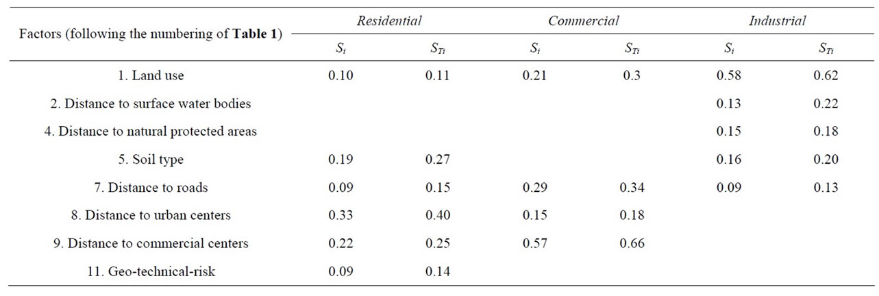
Table 3. Most significant factors in the SA, after introducing variations of ±25% for both factors and weights and considering the spatial variation of the model inputs.
simulating urban growth were: land use, distance to urban centers, distance to roads, distance to roads, commerce and hospitals, soil type and weighted distance for the most vulnerable population and that with purchasing power. However, a simplification of the model is not recommended. The model was executed only with the factors that drive the output variance of the model, but the results were rather different from the original. This means that, in order to improve the model, we have to pay special attention on these factors. We conclude that the model developed is robust and that it is not possible to simplify it without losing important parts of the final result.
Lastly, we would like to highlight the importance of carrying out this “partial validation” over the results of a prospective simulation model, where the comparison between model outputs and real data is impossible ([5] Paegelow and Camacho Olmedo, 2008). At least this kind of procedures can give some information about the robustness and consistency of the model and its results: First, because the methodology is simple and easy to be implemented in GIS, and second, because the proposed estimator (Si and STi) and the results are not affected greatly by changes made to the original variables of the model.
The SA is part of a validation procedure, and this information “would enable to inform policy makers, and other users of model results, on the uncertainties in the model outcomes and help the modeler to assess the suitability of the model for a particular situation and provide ideas to improve the model” ([3] Verburg, et al., 2004: 15). Thus, this type of study is very important because it helps on the development of new GIS-tools to assist in the simulation and analysis of future spatial models or alternative scenarios.
6. Acknowledgements
This research was performed in the context of SIMURBAN project (Analysis and Simulation of the urban growth using Geographic Information Technologies. Sustainability Evaluation), funded by the Spanish Ministry of Science (SEJ2007-66608-C04-00/GEOG).
REFERENCES
- J. I. Barredo and M. D. Gómez “Towards a Set of IPCC SRES Urban Land-Use Scenarios: Modeling Urban LandUse in the Madrid Region,” In: M. Paegelow and M. T. C. Olmedo, Eds., Modeling Environmental Dynamics. Advances in Geomatics Solution, Springer, Berlin, 2008, pp. 363-385.
- P. H. Verburg, P. P. Schot, M. J. Dijst and A. Veldkamp, “Land Use Change Modeling: Current Practice and Research Priorities,” GeoJournal, Vol. 61, No. 4, 2004, pp. 309-324. doi:10.1007/s10708-004-4946
- M. G. Delgado and J. Bosque Sendra, “Validation of GIS-performed analysis,” In: P. K. Joshi, P. Pani and S. N. Mohapatra, Eds., Geoinformatics for Natural Resource Management, Nova Science Publishers, Hauppauge, 2009, pp. 179-208.
- M. Paegelow and M. T. C. Olmedo, “Modeling Environmental Dynamics,” Springer-Verlag, Berlin, 2008.
- M. E. Qureshi, S. R. Harrison and M. K. Wegener, “Validation of Multi-Criteria Analysis Models,” Agricultural Systems, Vol. 62, No. 2, 1999, pp. 105-116. doi:10.1016/S0308-521X(99)00059-1
- M. L. Chu-Agor, R. Muñoz-Carpena, G. Kiker, A. Emanuelsson and I. Linkov, “Exploring Vulnerability of Coastal Habitats to Sea Level Rise through Global Sensitivity and Uncertainty Analyses,” Environmental Modeling & Software, Vol. 26, No. 5, 2011, pp. 593-604. doi:10.1016/j.envsoft.2010.12.003
- M. Crosetto, S. Tarantola and A. Saltelli, “Sensitivity and Uncertainty Analysis in Spatial Modeling Based on GIS,” Agriculture, Ecosystems and Environment, Vol. 81, No. 1, 2000, pp. 71-79. doi:10.1016/S0167-8809(00)169-9
- A. Saltelli, K. Chan and E. M. Scott, “Sensitivity Analysis,” Wiley, LTD., Chichester, 2000.
- A. Saltelli, M. Ratto, T. Andres, F. Campolongo, J. Cariboni, D. Gatelli, M. Saisana and S. Tarantola, “Global Sensitivity Analysis: The Primer,” Wiley, LTD., Chichester, 2008.
- A. Saltelli, S. Tarantola and K. Chan, “A Role for Sensitivity Analysis in Presenting the Results from MCDA studies to Decision Makers,” Journal of Multi-Criteria Decision Analysis, Vol. 8, No. 3, 1999, pp. 139-145. doi:10.1002/(SICI)1099-1360(199905)
- M. G. Delgado and J. B. Sendra, “Sensitivity Analysis in Multi-Criteria Spatial Decision-Making: A Review,” Human and Ecological Risk Assessment, Vol. 10, No. 6, 2004, pp. 1173-1187. doi:10.1080/10807030490887221
- C. J. Pettit, “Land Use Planning Scenarios for Urban Growth: A Case Study Approach,” Ph.D. Thesis, University of Queensland, Queensland, 2002.
- N. B. Chang, G. Parvathinathan and J. B. Breeden, “Combining GIS with Fuzzy Multi-Criteria Decision-Making for Landfill Sitting in a Fast-Growing Urban Region,” Journal of Environmental Management, Vol. 87, No. 1, 2008, pp. 139-153.
- P. Jankowski, “Integrating Geographic Information Systems and Multiple Criteria Decision Making Methods,” International Journal of Geographical Information Systems, Vol. 9, No. 3, 1995, pp. 251-273. doi:10.1080/02693799508902036
- S. Baja, D. M. Chapman and D. Dragovich, “Spatial Based Compromise Programming for Multiple Criteria Decision Making in Land Use Planning,” Environmental Model & Assessment, Vol. 12, No. 3, 2007, pp. 171-184. doi:10.1007/s10666-006-9059-1
- D. Geneletti and I. van Duren, “Protected Area Zoning for Conservation and Use: A Combination of Spatial MultiCriteria and Multi-Objective Evaluation,” Landscape and Urban Planning, Vol. 85, No. 2, 2008, pp. 97-110. doi:10.1016/j.landurbplan.2007.10.004
- L. Lilburne and S. Tarantola, “Sensitivity Analysis of Models with Spatially-Distributed Input,” International Journal of Geographic Information Systems, Vol. 23, No. 2, 2009, pp. 151-168.
- M. Crosetto and S. Tarantola, “Uncertainty and Sensitivity Analysis: Tools for GIS-Based Model Implementation,” International Journal of Geographical Information Science, Vol. 15, No. 5, 2001, pp. 415-437. doi:10.1080/13658810110053125
- M. G. Delgado and S. Tarantola, “Global Sensitivity Analysis, GIS and Multi-Criteria Evaluation for a Sustainable Planning of Hazardous Waste Disposal Site in Spain,” International Journal of Geographical Information Science, Vol. 20, No. 4, 2006, pp. 449-466. doi:10.1080/13658810600607709
- T. Wagener and J. Kollat, “Numerical and Visual Evaluation of Hydrological and Environmental Models Using the Monte Carlo Analysis Toolbox,” Environmental Modeling & Software, Vol. 22, No. 7, 2007, pp. 1021-1033. doi:10.1016/j.envsoft.2006.06.017
- Y. Tang, P. Reed, T. Wagener and K. van Werkhoven, “Comparing Sensitivity Analysis Methods to Advance Lumped Watershed Model Identification and Evaluation,” Hydrology and Earth system Sciences, Vol. 11, No. 2, 2007, pp. 793-817. www.hydrol-earth-syst-sci.net/11/793/2007/
- H. Varella, M. Guèrif and S. Buis “Global Sensitivity Analysis Measures the Quality of Parameter Estimation: The Case of Soil Parameters and a Crop Model,” Environmental Modeling & Software, Vol. 25, No. 3, 2010, pp. 310-319. doi:10.1016/j.envsoft.2009.09.012
- European Environment Agency (EEA), “Urban Sprawl in Europe, the Ignored Challenge,” EEA Report 10, Luxemburg, 2006.
- W. P. Rocha, M. G. Delgado and J. B. Sendra, “Land Use Changes and Urban Expansion in the Community of Madrid (1990-2000),” Scripta-Nova, Vol. XIII, No. 293, 2009. http://www.ub.es/geocrit/sn/sn-293.htm
- W. P. Rocha, M. G. Delgado and J. B. Sendra, “Development of Optimal Urban Growth Models for the Community of Madrid applying Multicriteria Evaluation Techniques and Geographic Information Systems,” GeoFocus (International Journal of Science and Technology of Geographic Information), Vol. 10, 2010, pp. 103-134. http://geofocus.rediris.es/2010/Articulo5_2010.pdf
- W. P. Rocha, M. G. Delgado and J. B. Sendra, “Simulating Urban Growth Scenarios Using GIS and Multi-Criteria Evaluation Techniques. Case Study: Madrid Region, Spain,” Environment and Planning B, Vol. 38, No. 6, 2011, pp. 1012-1031. doi:10.1068/b37061
- F. A. Benavente, W. P. Rocha, J. B. Sendra and M. G. Delgado, “Design and Simulation of Scenarios of Urban Land Demand in Metropolitan Areas,” International Journal of Sustainability, Technology and Humanism, Vol. 4, 2009, pp. 57-80. http://hdl.handle.net/2099/8535
- A. Saltelli, S. Tarantola and K. K. Chan, “A Quantitative Model Independent Method for Global Sensitivity Analysis of Model Output,” Technometrics, Vol. 41, No. 1, 1999, pp. 39-56. doi:10.2307/1270993
- R. I. Cukier, C. M. Fortuin, K. E. Schuler, A. G. Petschek and J. H. Schaibly, “Study of the Sensitivity of Coupled Reaction Systems to Uncertainties in Rate Coefficients. Part I: Theory,” Journal of Chemical Physics, Vol. 59, No. 8, 1975, pp. 3873-3878. doi:10.1063/1.431440
- M. Crosetto, J. A. M. Ruiz and B. Crippa, “Uncertainty Propagation in Models Driven by Remotely Sensed Data,” Remote Sensing of Environment, Vol. 76, No. 3, 2001, pp. 373-437. doi:10.1016/S0034-4257(01)00184-5
- M. Crosetto, F. Crosetto and S. Tarantola, “Optimized Resource Allocation for GIS-Based Model Implementation,” Photogrammetric Engineering & Remote Sensing, Vol. 68, No. 3, 2003, pp. 225-232.
NOTES
1We refer to factors and weights attached to the factors in the MCE techniques. We have to differentiate them from factors in SA. In the latter, factors include all the parameters of the model. In order to differentiate both, we will use variables instead of factors when talking about MCE techniques and we will use factors in the SA context.
2Software from the Institute for Systems, Informatics, and Safety at the Joint Research Centre of the European Union.