Natural Science
Vol.09 No.08(2017), Article ID:78836,38 pages
10.4236/ns.2017.98026
Using Earth’s Moon as a Testbed for Quantifying the Effect of the Terrestrial Atmosphere
Gerhard Kramm1, Ralph Dlugi2, Nicole Mölders3
1Engineering Meteorology Consulting, Fairbanks, AK, USA; 2Arbeitsgruppe Atmosphärische Prozesse (AGAP), Munich, Germany; 3Department of Atmospheric Sciences and Geophysical Institute, University of Alaska Fairbanks, Fairbanks, AK, USA
Correspondence to: Gerhard Kramm, ![]() ; Ralph Dlugi,
; Ralph Dlugi,  ; Nicole Mölders,
Copyright © 2017 by authors and Scientific Research Publishing Inc.
This work is licensed under the Creative Commons Attribution International License (CC BY 4.0).
http://creativecommons.org/licenses/by/4.0/


Received: August 7, 2017 Accepted: August 28, 2017 Published: August 31, 2017
ABSTRACT
In the past, the planetary radiation balance served to quantify the atmospheric greenhouse effect by the difference between the globally averaged near-surface temperature of and the respective effective radiation temperature of the Earth without atmosphere of resulting in . Since such a “thought experiment” prohibits any rigorous assessment of its results, this study considered the Moon as a testbed for the Earth in the absence of its atmosphere. Since the angular velocity of Moon’s rotation is 27.4 times slower than that of the Earth, the forcing method, the force-restore method, and a multilayer-force-restore method, used in climate modeling during the past four decades, were alternatively applied to address the influence of the angular velocity in determining the Moon’s globally averaged skin (or slab) temperature, . The multilayer-force-restore method always provides the highest values for , followed by the force-restore method and the forcing method, but the differences are marginal. Assuming a solar albedo of , a relative emissivity , and a solar constant of and applying the multilayer-force-restore method yielded and for the Moon. Using the same values for , , and , but assuming the Earth’s angular velocity for the Moon yielded and quantifying the effect of the terrestrial atmosphere by . A sensitivity study for a solar albedo of commonly assumed for the Earth in the absence of its atmosphere yielded , , and . This means that the atmospheric effect would be more than twice as large as the aforementioned difference of 33 K. To generalize the findings, twelve synodic months (i.e., 354 Earth days) and 365 Earth days, where , a Sun-zenith-distance dependent solar albedo, and the variation of the solar radiation in dependence of the actual orbit position and the tilt angle of the corresponding rotation axis to the ecliptic were considered. The case of Moon’s true angular velocity yielded and . Whereas Earth’s 27.4 times higher angular velocity yielded , , and . In both cases, the effective radiation temperature is , because the computed global albedo is . Thus, the effective radiation temperature yields flawed results when used for quantifying the atmospheric greenhouse effect.
Keywords:
Atmospheric Effect, Planetary Radiation Budget, Planetary Albedo, Effective Radiation Temperature, Skin Temperature, Slab Temperature, Forcing Method, Force-Restore Method, Multilayer-Force-Restore Method, Global Averaging

1. Introduction
The “thought experiment” of a planetary radiative equilibrium for the Earth in the absence of its atmosphere is considered to quantify the atmospheric effect (spuriously called the atmospheric greenhouse effect). The incoming flux of solar radiation, #Math_34#, that is absorbed at the Earth’s surface is given by [ 1 ]
(1.1)
Here, is the mean radius of the Earth considered as a sphere, is the solar constant, i.e., the total solar irradiance reaching the Earth’s surface for a mean distance (roughly 1 Astronomic Unit = AU) between the Sun’s center and the Earth’s orbit of (e.g., [ 2 , 3 ]), and is the planetary albedo of the Earth. Usually, a value for the solar constant close to is recommended (e.g., [ 4 - 6 ]), but recent satellite observations revealed a value of [ 7 - 10 ] (see Figure 1).

Figure 1. The 36-year record of the total solar irradiance (TSI) provided by different instruments (adopted from Kopp et al. [ 10 ], but updated).
Assuming a uniform temperature distribution on the Earth’s surface, i.e., temperature would be independent of longitude and latitude (note that this assumption is, by far, not fulfilled for the real Earth-atmosphere system), the total flux of infrared radiation emitted by the Earth’s surface, , as a function of this temperature and the planetary emissivity, , reads [ 1 ]
(1.2)
This equation is related to the power law of Stefan [ 11 ] and Boltzmann [ 12 ]. Assuming a so-called planetary radiative equilibrium, i.e., , yields (e.g., [ 1 - 5 , 13 - 16 ])
(1.3)
Commonly, Equation (1.3) is used to characterize the planetary radiation balance in the absence of the terrestrial atmosphere. Rearranging for temperature yields
(1.4)
This temperature value is called the “effective radiation temperature” of the Earth [ 1 ]. Assuming the Earth as a black body ( ) and using (e.g., [ 3 , 15 ]) and , Equation (1.4) leads to .
In case of the real Earth-atmosphere system, the global average of air temperatures observed close to the Earth’s surface at the stations of the global meteorological network and derived from data of weather satellites is . Consequently, the difference between this globally averaged temperature and the temperature of the planetary radiative equilibrium calculated by Equation (1.4) yields . Thus, it is stated that the so-called greenhouse effect of the terrestrial atmosphere causes a temperature increase of about . Kondratyev and Moskalenko [ 17 ], for instance, argued that their calculations for a standard model atmosphere yielded a total greenhouse effect of 33.2 K, with the following contributions from optically active gaseous components: H2O-20.6 K; CO2-7.2 K; N2O-1.4 K; CH4-0.8 K; O3-2.4 K; -0.8 K.
To our best knowledge, Equations (1.1) to (1.4) were introduced into the literature by [ 1 ] without adequate justification of their underlying assumptions. Assessment of these assumptions and their result of revealed [ 18 ]:
1) Only a planetary radiation budget of the Earth in the absence of an atmosphere is considered, i.e., any heat storage in the oceans (if at all existing in such a case) and land masses is neglected.
2) The assumption of a uniform surface temperature for the entire globe is rather inadequate. As shown by Kramm and Dlugi [ 19 ] this assumption is required by the application of the power law of Stefan [ 11 ] and Boltzmann [ 12 ] because this power law is determined by (a) integrating Planck’s [ 20 ] blackbody radiation law, for instance, over all wavelengths ranging from zero to infinity, and (b) integrating the isotropic emission of radiant energy by a small spot of the surface into the adjacent half space (e.g., [ 4 , 21 ]). These physical and mathematical reasons do not justify applying the Stefan-Boltzmann power law to a statistical quantity like . Even in the real situation of an Earth with atmosphere, (near-)surface temperatures vary notably from the equator to the poles owing to the varying solar insolation at the top of the atmosphere and from daytime to nighttime. Consequently, the assumption of a uniform surface temperature is inadequate. Our Moon, for instance, nearly satisfies the requirements of a planet without atmosphere. It has a non-uniform surface temperature distribution with strong variation from lunar day to lunar night, and from its equator to its poles (e.g., [ 22 - 26 ]). Furthermore, ignoring heat storage would yield a Moon surface temperature during lunar night of 0 K (or 2.7 K, the temperature of the space).
3) The choice of the planetary albedo of is rather inadequate. This value is based on satellite observations. Hence, it contains not only the albedo of the Earth’s surface, but also the back scattering of solar radiation by molecules (Rayleigh scattering), cloud and aerosol particles (Lorenz-Mie scattering). Budyko [ 27 ] already stated that in the absence of an atmosphere the planetary albedo cannot be equal to the actual value of (at that time, but today ). He assumed that prior to the origin of the atmosphere, the Earth’s albedo was lower and probably differed very little from the Moon’s albedo, which is equal to (at that time, but today ). A planetary surface albedo of the Earth of about is also suggested by the results of Trenberth et al. [ 28 ]. Thus, assuming a planetary albedo of and a planetary emissivity of (black body) in Equation (1.4) yields . For and , one obtains: . Haltiner and Martin [ 29 ] explained the so-called atmospheric greenhouse effect by the difference between the Moon’s surface temperature at radiative equilibrium and the globally averaged near-surface temperature of the Earth. They argued that the mean surface temperature of the Moon must satisfy the condition of radiative equilibrium so that (they used , , and , but this result is slightly too low).
4) Comparing with is rather inappropriate because the meaning of these temperatures is quite different. The former is based on an energy-flux budget at the surface even though it is physically inconsistent because of the non-uniform temperature distribution on the globe. Whereas the latter is related to globally averaging near-surface temperature observations made at meteorological stations (supported by satellite observations).
5) The Moon’s mean disk temperature of about 213 K retrieved at 2.77 cm wavelength by Monstein [ 30 ] is much lower than which can be derived with the Moon’s planetary albedo of . Even though the Moon’s mean disk temperature observed in 1948 by Piddington and Minnett [ 31 ] is about 26 K higher than that of Monstein [ 30 ], it is still 31 K lower than . Despite the Moon is nearly a perfect example of a planet without atmosphere, some authors argued that Equations (1.3) and (1.4) are only valid for fast-rotating planets so that the Moon must be excluded. Other authors, however, applied these equations for Venus that rotates a factor of four slower than the Moon. Pierrehumbert [ 32 ], for instance, used Equation (1.4) to calculate the temperature of the planetary radiative equilibrium for Venus. With and , he obtained . Chosing for the Venus in the absence of its atmosphere (which is similar to that of the Moon) yields and for as listed in NASA’s Venus Fact Sheet ( https://nssdc.gsfc.nasa.gov/planetary/factsheet/venusfact.html ) .
Because of these facts, we may conclude that Equation (1.4) is based on physically irrelevant assumptions and its results considerably disagree with observations. Consequently, the difference of lacks adequate physical meaning as do any contributions from optically active gaseous components calculated thereby.
In 2009, Gerlich and Tscheuschner [ 33 ] derived a globally averaged surface temperature of for the Earth in the absence of its atmosphere using the same assumptions commonly considered in deriving the effective radiation temperature except for the distribution of the surface temperature. Instead, they calculated surface temperatures for local radiative equilibrium. Their globally averaged surface temperature of is much lower than the effective radiation temperature of and, of course, much lower than the globally averaged near-surface temperature of . (Applying the formula of Gerlich and Tscheuschner [ 33 ] to the Moon would provide because ). Their calculation was performed for a non-rotating planet. Smith [ 34 ] confirmed their result for a non-rotating planet, but argued that on a rotating planet, the globally averaged surface temperature would be close to (or somewhat lower). If this result were correct, it would underline that the commonly accepted temperature difference of is not so far from reality. It seems, however, that Smith’s formula is affected by inappropriate averaging procedures [ 35 ]. Furthermore, in case of the Moon his formula would provide (or somewhat lower), a value close to its effective radiation temperature of , but much higher than the result of Monstein’s [ 30 ] observations of the Moon’s mean disk temperature. Because of this large discrepancy in the results of the globally averaged surface temperature and the consequence in evaluating the atmospheric effect, it is indispensable to assess whether the result of Gerlich and Tscheuschner [ 33 ] or that of Smith [ 34 ] is more relevant. Since Halpern et al. [ 36 ] did not consider observational evidence and previous model results regarding the Moon’s surface temperature and argued on the basis of Smith’s [ 34 ] result for a rotating airless planet, Smith’s result has to be assessed as well. Note that his manuscript was not published yet in a peer-reviewed scientific journal at that time. When Smith’s result is inappropriate for a rotating planet in the absence of its atmosphere the results of Kondratyev and Moskalenko [ 17 ] are insufficient as well.
Recently, Nikolov and Zeller [ 37 , 38 ] derived for the Moon, , and in a further step for an airless Earth, . Their results already suggested that neither the results of Gerlich and Tscheuschner [ 33 ] nor those of Smith [ 34 ] can be correct. Therefore, Equation (1.4) as well as the results of Gerlich and Tscheuschner [ 33 ], Smith [ 34 ], and Nikolov and Zeller [ 37 , 38 ] are assessed against the globally averaged surface temperature for a rotating globe without atmosphere, where, in addition, the tilt angle of the rotation axis to the ecliptic is considered.
The terrestrial atmosphere prevents to prove the “thought experiment” of a planetary radiative equilibrium on which Equation (1.4) for determining the effective radiation temperature is based. Fortunately, as aforementioned, our Moon nearly fulfills the requirements of a planet in the absence of its atmosphere because the density of the lunar atmosphere is so low that the exchange of heat between the top layer of the Moon’s regolith and its atmosphere can be neglected. The same is true in case of the down-welling infrared radiation even though traces of water vapor may occur in the lunar atmosphere. Thus, in recognition of previous surface temperature calculations performed for various areas of the Moon [ 22 - 26 , 39 ], we consider the Moon as a testbed for assessing the Equations (1.1) to (1.4) and the effect of the terrestrial atmosphere. With respect to Haltiner and Martin [ 29 ] as well as Budyko [ 27 ] the atmospheric effect is quantified by the difference between the global average of the air temperatures observed close to the Earth’s surface, , and the globally averaged surface temperature, , in the globally averaged surface temperature of the Moon. However, we must consider that the angular velocity of the Earth is 27.4 times higher than that of its Moon. Consequently, we performed our predictions for an airless planet rotating with a much higher angular velocity. In doing so, we adopted Budyko’s [ 27 ] suggestion that prior to the formation of the terrestrial atmosphere, the Earth’s surface and soil properties would probably be similar to those of the Moon.
2. Basic Considerations
2.1. The Globally Averaged Surface Temperature
Under consideration of the Earth’s true shape (the radius of the equator, 6378 km, is larger than the radius to the poles, 6356 km, owing to centrifugal forces), the average over the entire surface of the Earth reads [ 35 , 40 ]
(2.1)
Here, is an arbitrary variable, is the radius, is the solid angle of the entire planet, and is the differential solid angle, where and are the zenith and azimuthal angles, respectively, of a spherical coordinate frame (see Figure 2). Note that ranges from zero to , and ranges from zero to . For a spherical shape of the Earth as presupposed in deriving Equation (1.4), we have and . Thus, Equation (2.1) can be written as
(2.2)
Since the average along the parallel of latitude is given by
![]()
Figure 2. Mathematical representation of the solid angle. Here, is the differential solid angle, where and are the zenith and azimuthal angles, respectively (adopted from Kasten and Raschke [ 41 ]).
(2.3)
Equation (2.2) may also be written as
(2.4)
When we set, for instance, , the globally averaged surface temperature of a spherical planet in the absence of the atmosphere reads
(2.5)
The notion “surface temperature” is misleading. In his textbook, Planck [ 42 ] already stated:
“According to the principle of the conservation of energy, emission always takes place at the expense of other forms of energy (heat, chemical or electric energy, etc.) and hence it follows that only material particles, not geometrical volumes or surfaces, can emit heat rays. It is true that for the sake of brevity, we frequently speak of the surface of a body as radiating heat to the surroundings, but this form of expression does not imply that the surface actually emits heat rays. Strictly speaking, the surface of a body never emits rays, but rather it allows part of the rays coming from the interior to pass through. The other part is reflected inward and according as the fraction transmitted is larger or smaller the surface seems to emit more or less intense radiations.”
Bohren and Clothoaux [ 20 ] referred to Planck’s textbook and stated:
“Planck’s The Theory of Heat Radiation, an English translation of the second edition of which (1913) was published by Dover in 1959, is full of insights and qualifiers that have been forgotten over the years. For example, Planck recognized that ‘the surface of a body never emits rays, but rather it allows parts of the rays coming from the interior to pass through’ (p. 4), that a ‘finite amount of energy∙∙∙ is emitted only by a finite∙∙∙ volume, not by a single point’ (p.5)…”
From this point of view, the temperature has to be determined based on an energy budget for a thin slab adjacent to the surface at a certain location given by (see Figure 3)
![]()
Figure 3. Sketch of the energy exchange of a slab adjacent to the surface.
(2.6)
Here, is time, , , and , are the temperature, bulk density, and specific heat of this slab, respectively. The meaning of the “surface temperature” is, therefore, that of the slab or skin temperature. Furthermore, the symbol represents the various energy fluxes that are crossing the boundary of this slab represented by the surface , is the unit normal counted positive from inside to outside of the slab volume given by , where is the cross section, and is the thickness of this slab (see Figure 3).
The surface integral describes the exchange of energy between the volume of the slab and its surroundings. Since the transfer of energy through the lateral boundaries by heat conduction is rather inefficient, this transfer is usually ignored. This means that we only consider the exchange of energy at the top and bottom of this slab given by (see Figure 3)
(2.7)
Here, is the solar irradiance reaching the surface, is its reflected part, is the emitted infrared irradiance, is the soil heat flux density (simply called the soil heat flux), and are the normal units at the top and bottom of the slab, respectively. Since these normal units are functions of and or, alternatively, of and , where is the latitude, the scalar product is . Here, , and are the local zenith angle of the Sun’s center. Thus, the solar irradiance and its reflected part can be expressed as , where is the integral albedo of the solar range. Furthermore, the scalar product is given by , and that of by , where is the integral relative emissivity, and is the vertical component of the soil heat flux. The direction of is governed by the difference between the absorbed solar radiation and the emitted infrared radiation. Obviously, except , all quantities are functions of both and , where also depends on . Moreover, characterizes a possible gain or loss of energy inside of the volume owing to the conversion from one energy form to another. However, such energy conversion processes can be ignored when assuming dry soil.
Since is assumed to be independent of time, the l.h.s. of Equation (2.6) can be expressed by
(2.8)
where
(2.9)
is the volume average. Thus, Equation (2.6) may be re-written as
(2.10)
Ignoring the terrestrial soil heat flux, but considering the down-welling infrared radiation and the fluxes of sensible and latent heat, such an equation was already solved in UCLA general circulation model (GCM) by Arakawa [ 43 ] and in the GCM of the British Meteorological Office by Corby et al. [ 44 ] and Rowntree [ 45 ]. Deardorff [ 46 ] denoted this kind of equation the “forcing method”. Bhumralkar [ 47 ], Blackadar [ 48 ], and Deardorff [ 46 ] also inserted the terrestrial soil heat flux. Deardorff called this procedure the “force-restore method”. Bhumralkar [ 47 ] embedded his force-restore method in the two-level GCM of the Rand Corporation. A similar method is also used in various versions of ECHAM, the GCM of the Max Planck Institute for Meteorology at Hamburg, Germany, for both the land and sea areas (see, e.g., [ 49 - 51 ]). A surface has neither a mass nor a heat capacity. In addition, a surface cannot absorb or emit energy or exchange heat. Therefore, the temperature has to be considered as a representative temperature of the slab adjacent to the surface.
Under steady-state conditions, the l.h.s. of Equation (2.10) is zero. Thus, we have
(2.11)
This means that the slab, characterized by , , , and , does not further occur in the equation. Consequently, is replaced by the “surface temperature” .
Owing to the rotation of the planet, the slab temperature varies with time. Rearranging, for instance, Equation (2.11) yields
(2.12)
where depends on the temperature difference . Since both temperatures vary with time, the surface temperature, , can only be determined iteratively.
Inserting Equation (2.12) into Equation (2.3) yields
(2.13)
Thus, the integral in Equation (2.5) can be solved for an adequate number of averages along the parallel of any latitude. This equation yields then the true globally averaged surface temperature of the Earth in the absence of its atmosphere.
For the dark side of the Earth in the absence of its atmosphere, Equation (2.11) reduces to
(2.14)
Apparently, the soil heat flux links the surface temperature to the temperature at the outer edge of a heat reservoir within the soil. In the absence of a terrestrial atmosphere, this heat reservoir prevents the surface temperature from dropping to zero (or to the temperature of the space of about 2.7 K) during terrestrial night. If we assume, for instance, a surface temperature of on the dark side of the Moon and , the soil heat flux will amount to . Without this heat flux the predicted surface temperature on the dark side of the Moon would be equal to zero. Consequently, as argued by Gerlich and Tscheuschner [ 33 ], the soil heat flux has to be considered.
2.2. Soil Modeling
For the thin slab adjacent to the surface, for which uniform properties are assumed, may be expressed by the one-dimensional form of Fourier’s law of heat conduction (e.g., [ 22 , 24 , 39 , 52 - 56 ]),
(2.15)
related to the surface leads to
(2.16)
Here, is the soil temperature, and is the thermal conductivity. Wesselink [ 39 ], Jaeger [ 53 ], Cremers et al. [ 22 ], Mitchell and de Pater [ 52 ], and Vasavada et al. [ 24 , 26 ], for instance, used Equation (2.16) to predict the surface temperature for various areas on the Moon.
In accord with Equation (2.15), the soil heat flux in Equation (2.10) may be approximated by a finite difference scheme like
(2.17)
where is the soil temperature at depth below the slab, and . This soil temperature may still vary with time. To determine this temperature, the local balance equation for heat within the soil,
(2.18)
has to be solved. Here, is the soil temperature, and is the soil heat flux, and , again, are sources and sinks of heat owing to energy conversion within the soil. Again, is ignored because we only consider dry soil. Under this assumption, Equation (2.18) becomes a homogeneous parabolic differential equation. Furthermore, only the vertical transfer of heat is considered, i.e. is replaced by , where the vertical component is, again, expressed by . Since heat conductivity may vary with depth and temperature, the simplified version of Equation (2.18) reads [ 22 , 24 , 39 , 52 - 56 ]
(2.19)
To solve this parabolic differential equation, we have to consider not only initial conditions, but also boundary conditions. The lower boundary condition is customarily chosen in such a sense that at a certain depth the corresponding is constant with time during the period under consideration. This depth may be considered as the outer edge of a heat reservoir that is not notably affected by heat exchange. In case of the Moon, for instance, the results of Vasavada et al. [ 24 ] suggest that already in a soil depths of the variation of the temperature during one rotation of the Moon is negligible. Usually, a geothermal heat flux is considered at this depth, but its magnitude is of about . For most purposes this geothermal heat flux is negligible [ 52 ]. Since uncertainties due to unknown soil type distribution and properties notably exceed [ 57 , 58 ], no geothermal heat flux is considered in our calculations.
Figure 4 shows typical results at the lunar equator for a soil layer under the assumption of spatially
 (a)
(a)
 (b)
(b)
Figure 4. (a) Temperature and (b) heat flux of the upper regolith layer at the lunar equator. The calculations were performed for a period of using Equations (2.21) and (2.22).
and temporally constant bulk properties of regolith. The “surface temperature” is expressed by the harmonic function [ 59 , 60 ]
. (2.20)
Here, is the angular frequency, is the amplitude, is the period in seconds, and is the phase constant chosen as . The exact solution of Equation (2.19) is
(2.21)
In accord with Equation (2.15), the soil heat flux becomes
(2.22)
where is called the thermal skin depth [ 52 ], and is the thermal diffusivity. For , Equation (2.22) yields
(2.23)
Equation (2.21) demonstrates that the amplitude of the “temperature wave” decreases exponentially with increasing depth. The same is true for the heat flux wave described by Equation (2.22). In addition, the phases shift with increasing depth owing to .
The results in Figure 4 are based on , , , , , and that corresponds to the synodic month. Figure 4 illustrates the thermal environment of the upper lunar regolith during one period. Since the thermal skin depth depends on the angular frequency and, hence, on the rotation velocity, the calculation was also performed for a terrestrial day with a period of (Figure 5). As expected, the angular frequency increases because the period decreases. Consequently, the thermal skin depth is smaller leading to a stronger damping of the and signals than for . The increase of causes an additional phase shift between those two signals. Moreover, a small thermal skin depth yields a large soil heat flux at the surface, while the opposite is true for a thick thermal skin depth. Note that the
 (a)
(a)  (b)
(b)
Figure 5. As in Figure 4, but for a period of .
results illustrated in Figure 4 and Figure 5 also served to evaluate the numerical scheme described in the following and used in Subsections 6.3 and 6.4.
If the variation of the surface temperature is periodic, but not necessarily harmonic, the surface temperature may be expressed by a Fourier series as described, for instance, by Wesselink [ 39 ].
Cremers et al. [ 22 ], Mitchell and de Pater [ 52 ], Vasavada et al. [ 24 , 26 ], and Paige et al. [ 25 ] already used depth- and temperature-dependent regolith thermo-physical properties. Therefore, for the regolith bulk density, we use the formula of Vasavada et al. [ 26 ]
(2.24)
where and are the bulk densities close to the surface and at the depth , respectively. In earlier modeling activities, these bulk densities were considered for the top layer of a thickness of two centimeters and the entire layer below, respectively [ 24 , 52 ]. These activities applied a thermal conductivity of the form [ 24 , 52 , 61 ]
(2.25)
Here, is the phonon conductivity and is the ratio of “radiative” to phonon conductivity at a temperature of , where , and , were considered for the top layer and the layer below, respectively. Vasavada et al. [ 26 ] revised these formulas to
(2.26)
with , , and . The heat capacity as a function of the soil temperature reads
#Math_264# (2.27)
The formula for is based on the analysis of lunar soils samples from the Apollo landing sites Fra Mauro, Hadley-Appenine, and Descartes Highlands by Hemingway et al. [ 62 ], but their results are normalized by (see Figure 6). Wechsler et al. [ 63 ] recommended the exponential function for .
Since Moon’s regolith thermo-physical properties quantities, , , and , vary with depth and soil temperature, numerical solution of Equation (2.19) is indispensable. To integrate this equation, we introduce the variable transformation
. (2.28)
Here, is an arbitrary constant. Thus, the derivative of a quantity with respect to is
(2.29)
where . For our calculation, we use . Thus, Equation (2.19) reads
(2.30)
This variable transformation allows using central differences in even though the layer thickness increases with depth. The Crank-Nicolson scheme in combination with a Gauss-Seidel iteration procedure serve to numerical integrates this parabolic differential equation. These numerical techniques have already been used in the hydro-thermodynamic soil-vegetation scheme (HTSVS) developed by Mölders and Kramm (e.g., [ 54 , 55 , 58 , 65 - 67 ]). Despite the numerical techniques was thoroughly tested and evaluated by data from field campaigns during the development of HTSVS, we tested these techniques also against the results presented in Figure 4 and Figure 5 because of the drastic variation of Moon’s skin temperature. For our tests, we used an upper soil depth of , a maximum soil depth of and nine levels of equal intervals in of . Furthermore, we used the same values as considered in the analytical solution ( , , ). The “surface temperature” (Equation (2.20)) with and served as the upper boundary condition.

Figure 6. Temperature-dependent heat capacity of Moon’s soil. Data of the heat capacity taken from Robie et al. [ 64 ] and Hemingway et al. [ 62 ]. Note that the formula of Hemingway et al. [ 62 ] was rearranged for the normalized temperature (see Equation (2.27)), where .
Test results derived for the Moon are illustrated in Figure 7. With respect to the results of the analytical solution presented in Figure 4, only the relative numerical error of the soil temperature given by
and the numerical error of the soil heat flux given by
are illustrated, where the subscripts and denote the analytical and nu-
merical solutions, respectively. Note that is the arithmetic mean calculated for the layer between and for which the respective numerical solution was predicted.
2.3. Astronomical Aspects
The solar irradiance can be related to the solar constant by (e.g., [ 2 , 4 , 18 , 68 ])
(2.31)
where is the actual distance between the Sun’s center and the Earth’s center (or the Earth-Moon barycenter abbreviated by EMB) ranging from at the Perihelion and at the Aphelion, is the corresponding mean distance (roughly 1 AU) for which the solar constant is defined [ 4 , 29 ]. In case of the EMB, one may use Keplerian elements to predict [ 69 ]. Values of the Keplerian elements and their rates, with respect to the mean ecliptic and equinox of J2000, valid for the time-interval 1800 AD - 2050 AD are listed in Standish and Williams [ 70 ] (their Table 8.10.2). With respect to the position of the Moon, this procedure would lead to inaccurate results. Thus, we use the planetary and lunar ephemeris DE430 of the Jet Propulsion Laboratory (JPL) of the California Institute of Technology [ 71 , 72 ]. This ephemeris predicts both the actual distance between the Sun’s center and the Earth’s center, , and that between the Sun’s center and the Moon’s center, . We used the JPL Fortran subroutine PLEPH to calculate and . Typical results computed for a period of 354.4 terrestrial days
 (a)
(a)
 (b)
(b)
Figure 7. (a) Relative numerical error in percent of the numerically predicted soil temperature with respect to the analytically derived soil temperature ; (b) Numerical error of the numerically predicted soil heat flux with respect to the arithmetic mean of the corresponding analytical solutions and for the layer between and .
starting with January 15, 2010, 11:07 UT1 (Barycentric Dynamical Time , New Moon) are illustrated in Figure 8. Note that this period is embedded in the 800 days-period of Vasavada et al. [ 26 ] that starts with . Thus, their results may be considered for comparison. Using Equation (2.31) and the values of and , we also predicted the corresponding TSI reaching the respective sub-solar point either of the Moon or Earth (Figure 8).
In 2010, the geocentric distance of the Moon varies from 356,593 km at Perigee to 406,540 km at Apogee with an average distance of 384,767 km. Compared with the heliocentric position of the EMB, an additional variation of the actual distance between the Sun’s center and the Moon of 763133 km occurs (Figure 8). Thus, the solar irradiance reaching the surface of the Moon at the sub-solar point depends on Moon’s actual heliocentric distance, rather than on the heliocentric distance of the EMB. Based on Equation (2.31), this solar irradiance varies by ( ) comparable with the soil heat flux shown in Figure 4. Consequently, Moon’s actual heliocentric distance should not be replaced by that of the EMB when predicting the skin temperature at a given location of the Moon.
The Earth-atmosphere system and the Moon not only reflect solar radiation, but also emit infrared radiation to space. Of course, these facts would be also true for an Earth in the absence of its atmosphere. When we assume, for instance, that at the sub-terrestrial point (also called the Sub-Earth point) of the Moon, the sum of the reflected solar radiation and emitted infrared radiation in the direction of the sub-lunar point of the Earth would amount to a maximum value of , the radiative effect on the sub-lunar point of the Earth, , would be , according to
. (2.32)
Here, is the mean radius of the Moon, and is the distance at Perigee ( ). On the contrary, considering at the sub-lunar point of the Earth in the absence of its atmosphere and replacing by the mean radius of the Earth, , would yield a radiative effect, , on the sub-terrestrial point of the Moon of about
 (a)
(a)
 (b)
(b)
Figure 8. Variation of (a) the distance between the Sun’s center and the Moon’s center, rM, as well as between the Sun’s center and the Earth’s center, r, determined for a period of 354 days starting with January 15, 2010, 11:07 UT1 ( , New Moon) as obtained by the JPL planetary and lunar ephemerides DE430, and (b) the TSI reaching the sub-solar point either of the Earth (at the top of the atmosphere) or the Moon, where Equation (2.31) and were used.
. These radiative effects are in the range of uncertainty [ 57 , 58 ], for which they were neglected in our study.
The function can be determined using the rules of spherical trigonometry (e.g., [ 2 , 4 , 18 , 68 ]). For Earth, one obtains
(2.33)
Here, is the declination of the Sun, is latitude, and is the hour angle from the local meridian. The solar declination angle is related to
, (2.34)
where is the oblique angle, and is the true longitude of the Earth counted counterclockwise from the vernal equinox (e.g., [ 2 , 4 , 18 , 68 , 69 ]), is the true anomaly, i.e., the positional angle of the Earth on its orbit counted counterclockwise from the Perihelion, and is the longitude of the Perihelion counted counterclockwise from the moving vernal equinox. For Earth, ranges from 23˚27'S (Tropic of Capricorn; ) to 23˚27'N (Tropic of Cancer; ), and ranges from to , where represents the half-day, i.e., from sunrise to solar noon or solar noon to sunset The half-day can be deduced from Equation (2.33) by setting (invalid at the poles) leading to . In our study, we predicted based on the DE430 data. For the Moon, has to be replaced by the selenographic latitude, , of the Sun.
In accord with Taylor et al. [ 73 ], we computed, among others, the selenographic longitude, , and the selenographic latitude, , using
(2.35)
and
(2.36)
where is the inclination of the ecliptic to the mean lunar equator adopted from Newhall and Williams [ 74 ], is the ascending node of Moon’s orbit on the ecliptic adopted from Folkner et al. [ 72 ], is the mean longitude of the Moon adopted from Simon et al. [ 75 ], and is the nutation in longitude. The selenographic colongitude is given by . Furthermore, the heliocentric ecliptic latitude and longitude of the Moon, and , can be determined by
(2.37)
and
. (2.38)
Here, is the heliocentric vector to the Moon, where is its length. The respective data are provided by DE430. The results obtained for and are illustrated in Figure 9.
3. The Equation of Gerlich and Tscheuschner
Ignoring , and assuming and as constant for the entire globe in Equation (2.11) yields
. (3.1)

Figure 9. Variation of the declination, δS, and the selenographic latitude, bS, of the Sun determined for a period of 354 days starting with January 15, 2010, 11:07 UT1 ( , New Moon) as obtained by the JPL planetary and lunar ephemerides DE430.
This local radiative balance leads to the local surface temperature
. (3.2)
Inserting Equation (3.2) into Equation (2.2) and setting yield
(3.3)
or with respect to Equation (1.4)
(3.4)
The simplest solution of Equation (3.4) can be obtained by assuming . Since does not vary more than 3.5 percent [ 4 , 18 ], it is frequently assumed that . This simplification yields
(3.5)
with and
(3.6)
where the imaginary unit is defined by . Since temperature is a real quantity, one finally obtains (see [ 33 ])
(3.7)
Smith [ 33 , 34 ] confirmed this result already for a non-rotating planet. As stated by Gerlich and Tscheuschner [ 33 ], Equation (3.7) satisfies the requirement of Hölder’s [ 76 ] inequality that results in , where, however, the true value of is unknown because of the uncertainty with which especially the values of the planetary albedo and planetary emissivity are fraught. As aforementioned, assuming , , and yields an effective radiation temperature of the Earth of . Equation (3.7), however, provides [ 33 , 34 ], i.e., the condition of a non-rotating globe, as assumed in the “thought experiment” of a planetary radiation balance for the Earth in the absence of an atmosphere, leads to a globally average temperature, , which is 111 K lower than . Note that using produces only a small deviation of 0.3 K.
For (valid for both the vernal equinox and the autumnal equinox), Equation (2.33) provides , i.e., a rotating planet is considered. In case of the vernal equinox, the distance of the EMB would be and, hence, . However, for comparability, we use the common assumptions and . Thus, Equation (3.2) becomes
(3.8)
Figure 10(a) illustrates results of the diurnal variation of for various parallels of latitude provided by Equation (3.8). Using Equation (2.5) yields . Thus, Gerlich and Tscheuschner’s result for a non-rotating Earth in the absence of its atmosphere holds for a rotating one.
The solar radiation absorbed, , for the same parallels of latitude is shown in Figure 10(b). Using Equation (2.4) for determining the global average of the absorbed solar radiation yields . This value substantially agrees with that was used for determining the effective radiation temperature of . Note that is ba-
 (a)
(a)
 (b)
(b)
Figure 10. Variation of the (a) surface temperature and (b) absorbed solar radiation for numerous parallels of latitude in case of the Earth in the absence of its atmosphere.
lanced by the globally averaged infrared radiation. Thus, the result of Gerlich and Tscheuschner [ 33 ] of is correct as long as the heat transfer and heat reservoir within the soil are ignored as done in deriving Equation (1.4). Under these conditions, Halpern et al. [ 36 ]’s criticism regarding this globally averaged temperature becomes obsolete.
The results in Figure 10 demonstrate that under the same global average of the absorbed solar radiation quite different surface temperature distributions are possible. These different surface temperature distributions lead to different global averages of the surface temperature for the Earth in the absence of its atmosphere: The uniform surface temperature distributions leads to an effective radiation temperature of . Whereas the distribution of the surface temperature that is governed by a local radiative balance Equation (3.1) provides a global average surface temperature of .
As mention in Section 1, using is inadequate because this value is only valid for the entire system Earth-Atmosphere. Here two-thirds of this value have to be attributed to the atmosphere. In addition, the assumption is questionable. If we consider and the optical properties for the Moon [ 26 ] of and , Equation (1.4) will provide for the effective radiation temperature of the Earth in the absence of its atmosphere (and of the Moon) of , where . In this case, Formula (3.7) yields . Based on the local radiative balance Equation (3.1), Equation (3.8) as well as Equations (2.3) and (2.4) we also obtain . Then, the global average of the absorbed solar radiation amounts to and is balanced by the globally averaged emitted infrared radiation as well.
The results provided by the Diviner Lunar Radiometer Experiment onboard the Lunar Reconnaissance Orbiter, however, suggest an equatorially averaged surface temperature of 215.5 K with an average maximum of 392.3 K and average minimum of 94.3 K [ 77 ]. This means that the local thermal effect of the soil must be considered.
4. Smith’s Equation
The basic equation of Smith [ 34 ] reads
(4.1)
Here, is the thermal inertia coefficient (heat capacity times the thickness of the layer under study), is the temperature representative for the layer under study for which the thermal inertia coefficient has to be determined, is the position vector represented by the longitude, , and the latitude, , is the albedo, is the surface temperature, and and are the absorbed solar radiation and emitted terrestrial radiation, respectively. Furthermore, is a step function with which the incoming solar radiation is weighted. In principle, Equation (4.1) corresponds to Equation (2.10), i.e., the temperature is a volume-averaged quantity. Smith also assumed that the soil heat flux is generally negligible. This means that this equation corresponds to the forcing method.
Following Smith [ 34 ], the solar zenith distance is related to
. (4.2)
Here, is the period of one rotation. For simplification, he set so that with . For , Equation (2.33) provides
(4.3)
i.e., Smith assumed . His step function reads
(4.4)
Integrating Equation (4.1) yields
(4.5)
or
(4.6)
By assuming and defining an effective surface temperature, , according to the time average,
(4.7)
Smith obtained
(4.8)
Inserting Equation (4.8) into Equation (2.2) yields
(4.9)
Smith also assumed and obtained the same results like for a non-rotating planet because the assumption of in Equation (1.4) yields
(4.10)
The drawbacks and insufficiency of this equation were already discussed in detail in Section 1. Recall that generally , i.e., and have different meanings.
5. The Analytical Model of Nikolov and Zeller
The so-called analytical model of Nikolov and Zeller [ 37 , 38 ] is based on a formula like Equation (2.12), but is written as
(5.1)
where is the fraction of solar radiation stored into Moon’s regolith through heat conduction. The authors included cosmic microwave background radiation (CMBR), but neglected it later as it is very small. Inserting formula (5.1) into Equation (2.2) provides
(5.2)
By ignoring also , they finally proposed
(5.3)
where and is an effective value for . Nikolov and Zeller stated:
“Conceptually is a non-dimensional thermal enhancement factor that boosts the global temperature of an airless planet above the level expected from a surface with zero thermal inertia, i.e. if the planet were completely non-conductive to heat.”
They proposed for their thermal enhancement factor
(5.4)
Comparing Equation (3.7) with Equation (5.3) provides . Since Gerlich and Tscheuschner [ 33 ] excluded any soil effects, one may conclude . This condition would require .
Nikolov and Zeller [ 37 , 38 ] derived a value of for Moon’s globally averaged surface temperature and a similar value for the Earth ranging from to . For the validation of their analytical model, Nikolov and Zeller fitted modeled latitudinal temperature averages with a sixth-order polynomial. These modeled latitudinal temperature averages are based on the predictions of Vasavada et al. [ 26 ] for the Moon with NASA’s TWO model. This thermo-physical model of the regolith is based on the diagnostic Equation (2.11) that has to be solved iteratively, and the prognostic Equation (2.19). The depth- and temperature-dependent regolith thermo-physical properties used by Vasavada et al. [ 26 ] are described by Equations (2.24), (2.26), and (2.27).
6. The Globally Averaged Slab Temperature for a Rotating Planet in the Absence of an Atmosphere
As aforementioned, the Earth’s Moon nearly fulfills the requirements of a planet that has no atmosphere. Therefore, we considered the Moon to test the truth or falsehood of the effective radiation temperature as a representative quantity for the true globally averaged surface temperature.
In contrast to various authors (e.g. [ 22 , 24 , 26 , 39 , 52 , 53 ]) who predicted the surface temperature of various areas on the Moon using the diagnostic Equation (2.11), we integrated the prognostic Equation (2.10) for determining the globally averaged slab temperature of the Moon for a synodic month ( ). In doing so, we used Gear’s [ 78 ] numerical algorithm DIFSUB. Following Budyko [ 27 ], we assumed that prior to the origin of the terrestrial atmosphere, the Earth’s soil properties would probably differ little from those of the Moon. Thus, the main difference between the Moon and the Earth in the absence of its atmosphere is the huge difference in the angular velocities of their rotation. Therefore, we integrated Equation (2.10) also for a terrestrial day ( ). (Note that in the absence of the terrestrial atmosphere, oceans cannot exist because in case of oceans, at least, a water vapor atmosphere would exist leading, at least, to a downwelling infrared radiation and a latent heat flux.) There are two reasons to use the prognostic Equation (2.10). First, it permits addressing the impact of the angular velocity. Second, such a prognostic equation has been used in GCMs during the past four decades, where, of course, the down-welling infrared radiation and fluxes of sensible and latent heat were included.
6.1. The Forcing Method
First, we approximated the prognostic Equation (2.10) in the concept of the forcing method, which was used, for instance, in UCLA’s GCM by Arakawa [ 43 ] and in the GCM of the British Meteorological Office by Corby et al. [ 44 ] and Rowntree [ 45 ]. This method ignores the soil heat flux. Thus, this equation was rearranged to
(6.1)
with , , and . The latter is, again, the thermal inertial coefficient. For the Moon, we used , , and . This thickness of the slab corresponds to an average value of the thermal skin depth . For , the thermal skin depth amounts to an average value of 0.01 m, as in Bhumralkar [ 47 ]. Because of the regolith thermo-physical properties of the Moon, we used, however, a thickness of the slab of and, hence, . Even though the distance between the Sun and Moon and, hence, the TSI notably varies during a synodic month (see Figure 8), we expressed by the solar constant , i.e., the actual distances between the Sun’s center and the Earth and its Moon is replaced by a mean distance (see Equation (2.31)). To compare the Moon’s effective radiation temperature of with the corresponding globally averaged temperature we used, at first, the following simplifications: The effect of Moon’s axial tilt of about 1.54˚ with respect to the normal vector of the ecliptic plane is neglected yielding . Moreover, we assumed and .
Figure 11 shows the results of our integrations for a synodic month ( ) and terrestrial day ( ). These results yield a globally averaged slab temperature of for and of for . This notable temperature difference is related to the huge difference in the angular velocities of Earth and Moon. For one complete rotation of a celestial body, the soil surface is longer exposed to solar radiation for low than high angular velocity. Consequently, under slow rotation, a surface gains more heat yielding to increased soil heat flux compared to a fast rotating celestial body―both without atmosphere―if their soil properties are equal. During the long night, more heat is released to space under slow than fast rotation.
Nevertheless, both globally averaged slab temperatures are much lower than the aforementioned effective radiation temperature of the Moon. For , the difference is . For , it is . This means that the difference between the globally averaged near-surface temperature, , and the globally averaged slab temperature of the Earth in the absence of its atmosphere would be . This difference may be attributed to the effect caused by the terrestrial atmosphere. This value is 1.93 times larger than the temperature difference of 33 K commonly attributed to the atmospheric-greenhouse effect under consideration of the effective radiation temperature of the Earth in the absence of the terrestrial atmosphere.
 (a)
(a)
 (b)
(b)
Figure 11. The variation of the slab temperature for numerous parallels of latitude for the Moon as provided by the forcing method for periods of (a) and (b) . The predictions were performed using the forcing method.
Our results provided an average surface temperature along Moon’s equator of . This value is 8.1 K lower than the equatorially averaged surface temperature of the Moon of 215.5 K provided by the Diviner Lunar Radiometer Experiment [ 77 ]. Our value of for is notably larger than the 197.3 K derived for Moon’s globally averaged surface temperature and the similar value for the Earth by Nikolov and Zeller [ 37 , 38 ].
The globally averaged absorbed solar radiation used for determining the effective radiation temperature of the Moon is given by . The results of the forcing method provide for and for , respectively. These values are balanced by the globally averaged emitted infrared radiation, , as well. As mentioned in Section 3, these values were also related to Equation (3.7) even though this equation yields a globally averaged surface temperature of and for the Moon and Earth (in absence of its atmosphere), respectively. This means that quite different skin temperature distributions are possible even though the globally averaged fluxes of absorbed and emitted radiation are identical.
Since the angular velocity of the Earth is much higher than that of the Moon, the response time of the emitted infrared radiation with respect to the absorbed solar radiation causes different effects (Figure 12). Obviously, the model has to be spun up to equilibrium prior to analysis of the results [ 79 ]. For we predicted always three days, where the results obtained for the first day slightly differs from those of the second and third day. Thus, we discarded the first two days when calculating the global-averages.
It is well-known (e.g. Pielke [ 79 ]), that any diagnostic procedure requires quasi-equilibrium conditions at the location of interest. In case of surface temperature and fluxes, the condition of quasi-equilibrium is more likely for slow than fast rotation. Consequently, the diagnostic procedure given by Equation (2.11) seems to be suitable only for the Moon.
6.2. The Force-Restore Method
Next, we inserted the soil heat flux into Equation (2.10) in the concept of the force-restore method (e.g. [ 46 - 48 ]). Thus, Equation (6.1) becomes
(6.2)
 (a)
(a)
 (b)
(b)
Figure 12. The response time of the emitted infrared radiation with respect to the absorbed solar radiation for both (a) and (b) exemplarily shown for the respective equator. The predictions were performed using the forcing method.
with and as before, and , where is the soil temperature at the depth below the slab leading to a difference of (see Equation (2.17)). Again, was used. Soil temperatures at the depth were considered as constant over one rotation, but varied with latitude. These values were approximated from the temperature distribution proposed by [ 24 ]. The results illustrated in Figure 4 and Figure 21 underlined that is an appropriate choice.
Equation (6.2) corresponds to Deardorff’s [ 46 ] formula (8a) except for his constants and that served to yield the exact solution for a sinusoidally varying soil surface heat flux after any transients have died away. Since there is no sinusoidal behavior for and , we set them to zero.
Again, we assumed , , and as well. As exemplarily shown in Figure 13 for the respective equator, the results provided by the force-restore method yields marginally higher minimum temperatures than those provided by the forcing method. For both the Moon and Earth in absence of its atmosphere, the energy loss due to the emission of radiation is reduced by the soil heat flux when the force-restore method is applied. For the force-restore method, the response time of the emitted infrared radiation with respect to the absorbed solar radiation is comparable with that of the forcing method (Figure 12). The respective soil heat fluxes are shown in Figure 14. As expected, for , the magnitude of the soil heat flux is relatively small, while it is notably larger for .
The force-restore method provides a globally averaged slab temperature of for and of for . The differences between the effective radiation temperature of the Moon and the globally averaged slab temperature are for and for , respectively. With respect to obtained for , the effect caused by the terrestrial atmosphere would be . It is 0.4 K smaller than for the forcing method.
The globally averaged absorbed solar radiation is for and for , respectively. Again, these values agree well with used in deriving the effective radiation temperature of the Moon. Note that the values of the globally averaged emitted infrared radiation, , are slightly lower than those of the absorbed solar radiation so that radiative imbalances of about to occur. This uncertainty is not surprising because the prediction of the soil heat flux is relatively crude in the force-restore method. However, these discrepancies are compensated by the globally averaged values of the soil heat flux .
 (a)
(a)
 (b)
(b)
Figure 13. Difference in the slab temperatures at the equator between the forcing method, the force-restore method, and the multilayer-force-restore method as obtained for the Moon for (a) and (b) .
 (a)
(a)
 (b)
(b)
Figure 14. The variation of the soil heat flux for numerous parallels of latitude for the Moon, where periods of (a) and (b) were considered. The results were provided by the force-restore method.
In case of , we also predicted the globally averaged slab temperature also for because the effective radiation temperature of for the Earth in the absence of its atmosphere is based on a planetary albedo of (Figure 15). The respective globally averaged temperature and the absorbed solar radiation amount to and, again, , respectively (Figure 16). For , the difference between the effective radiation temperature and the globally averaged slab temperature is . Again, is about lower than , but compensated by the globally averaged soil heat flux. With respect to obtained for , the effect of the terrestrial atmosphere would be . This value is 2.2 times larger than the 33 K commonly considered.
6.3. The Multilayer-Force-Restore Method
To further improve the calculation of the soil heat flux, we coupled the force-restore method with the multilayer numerical model of Moon’s regolith described in Subsection 2.2. For ease of readability, we call this coupled model the multilayer-force-restore method hereafter. For this coupling procedure, we made the following changes in Equation (6.2). Now, is the time-dependent temperature of the first level below the slab at the depth of . Then is given by with . In contrast to the tests of the numerical scheme (Subsection 2.2, we used 16 levels in our computations and . The latter is more suitable in long-term predictions, where the temperature at this depth, , is considered as constant, but dependent on latitude. Again, we used the approximated temperature distribution of [ 24 ].
Technically, the numerical solution of the multilayer-force-restore method is a semi-implicit coupling [ 79 ]. This means the soil heat flux was predicted by using the slab temperature provided by Equation (6.2) at the previous time step. Then, this soil heat flux served to predict the slab temperature at the following time step. A time step of 600 s was used. The coupled model was spun up to quasi-steady-state vertical profiles of the soil temperature prior to starting the predictions of the slab temperature and the temperature and the heat flux within the deeper regolith.
A slab thickness of , as used by both the forcing method and the force-restore method for , would yield an equatorially averaged slab temperature of , which is notably higher than 215.5 K provided by the Diviner Lunar Radiometer Experiment [ 77 ]. However, in contrast to these
 (a)
(a)
 (b)
(b)
Figure 15. Variation of slab temperature and soil heat flux for numerous parallels of latitude for a terrestrial day of and . The results were provided by the force-restore method.
 (a)
(a)
 (b)
(b)
Figure 16. The terms and as required by Equation (2.5), where and are the averages of the surface temperature and the absorbed solar radiation along the parallel of latitude, respectively. The results were provided by the force-restore method (see Equation (6.2)) for different values of the solar albedo . The green line represents the results provided by Equation (3.8).
method, which were based on an averaged thermal skin depth, the multi-layer force-restore method expresses this depth by multiple layers. Consequently, it permits consideration of vertical temperature and soil heat flux gradients. To take full advantage of this improved approach, we reduced the “slab thickness” to . Doing so yields an equatorially averaged slab temperature of for and (Figure 13), and for a Sun-zenith-dependent variable solar albedo (Equation (6.3)) and . Note that the latter is comparable with that of [ 26 ].
The minimum temperatures obtained by the multilayer-force-restore method are 104.5 K for and 99.4 K for and , and 97.5 K for and a Sun-zenith-dependent solar albedo (Equation (6.3)) and . Both minimum temperatures obtained for seem to be more appropriate than those obtained by the forcing method or force-restore method.
Recall, the force-restore method provided a minimum temperature of 57 K and an equatorially averaged temperature of 196.7 K for and at (Figure 13). Together, these results demonstrate that for the Moon a thickness of the slab of may be advantageous for the forcing method and the force-restore method, but is more appropriate for the multilayer-force-restore method. Note that for these reasons and to take full advantage of the multi-layer force restore method, we used in the simulations with the multilayer-force-restore method for both and .
Figure 17 illustrates the results provided by the multilayer-force-restore method, where, again, , , and were used for comparison with the effective radiation tempera-
 (a)
(a)
 (b)
(b)
 (c)
(c)
 (d)
(d)
Figure 17. Variation of the slab temperature for numerous parallels of latitude for the Moon for (a) and (b) , and the soil heat fluxes for (c) and (d) as provided by the multilayer-force-restore method.
ture. We obtained for and of for yielding for and for . In case of , the effect of the terrestrial atmosphere is , i.e., 1.8 times larger than the 33 K commonly considered.
The globally averaged absorbed solar radiation is for and for . In these instances, the values of the globally averaged emitted infrared radiation are marginally higher than those of the absorbed solar radiation and compensated by the globally averaged soil heat fluxes.
Like for the force-restore method, we also performed a sensitivity study assuming . We obtained and, again, , respectively. For , the difference between the effective radiation temperature and the globally averaged slab temperature is . Again, slightly exceeds . This marginal radiative imbalance is compensated by the globally averaged soil heat flux. With respect to , the difference between the globally averaged near-surface temperature and the globally averaged slab temperature of the Earth in the absence of its atmosphere would be . This value is 2.1 times larger than the 33 K commonly related to the atmospheric effect.
6.4. Generalization of the Results
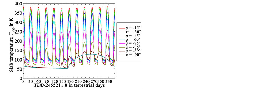
To generalize our findings, we considered for the Moon twelve synodic months, i.e., 354.4 terrestrial days, starting with TDB = 2,455,211.8 (January 15, 2010, 11:07 UT1, New Moon). In case of the 27.4 times higher angular velocity of the Earth, our numerical simulations covered 365.26 terrestrial days starting with TDB = 2,455,197.5 (January 1, 2010, 00:00 UT1). Two numerical simulations were performed, one with the force-restore method and one with the multilayer-force-restore method. In both simulations, we used a local emissivity of and a local solar albedo expressed by Keihm’s [ 80 ] empirical formula (slightly rearranged)
(6.3)
where is the local zenith angle of the Sun’s center, is the normal albedo, and and are empirical values. With exception of Keihm’s value for , all others are based on observations of the Lunar Reconnaissance Orbiter Diviner Lunar Radiometer Experiment (see [ 25 , 26 ]).
Results provided by the multilayer-force-restore method (Figure 18) exhibit effects by (a) the variation of the TSI owing to Moon’s distance from Sun’s center and (b) the variation of the selenographic latitude of the Sun. Figure 19 shows results of these predictions in more detail for the synodic month started at TDB = 2,455,521.9. Also illustrated are the zonal mean bolometric temperatures and the standard deviation versus local time for numerous parallels of latitude provided by the Diviner Lunar Radiometer Experiment [ 77 ]. Obviously, the model results well agree with the observations.
The corresponding solar radiation, absorbed solar radiation, and emitted infrared radiation averaged over terrestrial days are exemplarily shown in Figure 20 for two different synodic months. These results for the slab temperatures only differ marginally from each other indicating that the model well captures the conditions over the time frame of the orbit around Sun. The same is true in case of the soil heat flux. The force-restore method provided similar pattern for the slab temperature (therefore not shown), but with notably different soil heat fluxes due to their crude parameterization. The vertical distributions of temperatures and heat fluxes within Moon’s regolith for these two different synodic months are exemplarily shown in Figure 21 for the equator and the latitude 75˚N. Again, the respective results only differ marginally from each other.
The results illustrated in Figure 18 yield a globally averaged slab temperature of for twelve synodic months. The globally averaged solar radiation reaching Moon’s surface is
, because twelve synodic months do not completely cover the entire orbit of the
 (a)
(a)
 (b)
(b)
Figure 18. Variation of the slab temperature for numerous parallels of latitude by the multilayer-force-restore method for Moon’s (a) northern and (b) southern hemisphere for twelve synodic months, starting with TDB = 2455211.8 (January 15, 2010,11:07 UT1, New Moon).
 (a)
(a)
 (b)
(b)
 (c)
(c)
 (d)
(d)
Figure 19. (a) Zonal mean bolometric temperatures and (b) standard deviation versus local time for numerous parallels of latitude (adopted form Williams et al. [ 77 ]). Also shown are model results provided by the multilayer-force-restore method for the synodic month started at TDB = 2455521.9 for the (c) northern hemisphere (including the equator) and (d) southern hemisphere.

Figure 20. Comparison of two different synodic months for daily mean solar radiation at the (a) beginning and (b) close to the end of an orbit around Sun, for daily mean absorbed solar radiation at the (c) beginning and (d) close to the end of an orbit around Sun, and for daily mean emitted infrared radiation at the (e) beginning and (f) close to the end of an orbit around Sun. The numerical simulations were performed for twelve synodic months starting with TDB = 2455211.8 (January 1, 2010, 00:00 UT1).
 (a)
(a)
 (b)
(b)
 (c)
(c)
 (d)
(d)
 (e)
(e)
 (f)
(f)
 (g)
(g)
 (h)
(h)
Figure 21. The vertical distribution of the temperature and the heat flux within Moon’s regolith for two different synodic months at the equator ((a) to (d)) and for the latitude 75˚N ((e) to (h)) at the beginning and close to the end of an orbit around Sun. The numerical simulations were performed for twelve synodic months starting with TDB = 2,455,211.8 (January 1, 2010, 00:00 UT1).
Earth-Moon barycenter around the Sun. As the globally absorbed solar radiation amounts to , the global albedo in the solar range is about . For , the effective radiation temperature is . Thus, the difference between the effective radiation temperature and the globally averaged skin temperature is . For comparison: The force-restore method yielded and .
The globally emitted infrared radiation is . Thus, there is a slight radiative imbalance of . This small imbalance corresponds to the globally averaged soil heat flux as well. Even though this small value plays no role in the global energy budget of the Moon, it does not mean that the local thermal effect of the regolith is negligible, too. Excluding, for instance, this local thermal effect would lead to Equations (3.1) and (3.2) and, hence, to a globally averaged surface temperature of . Using Equation (3.7) yields .
The results of our numerical simulations using the multilayer-force-restore method for the 27.4 times higher angular velocity of the Earth are illustrated in Figure 22. Part (a) of this figure shows the daily mean slab temperature as a function of latitude and terrestrial day of the year. Based on this temperature distribution, we obtained a globally averaged slab temperature of . Thus, the difference between the effective radiation temperature of (obtained with and ) the globally averaged slab temperature is . With respect to the value of , we obtain , which is twice as large as the 33 K commonly considered as atmospheric effect. For comparison: The force-restore method provided , , and .
Figure 22 also shows the (b) daily mean values of solar radiation, (c) absorbed solar radiation, (d) emitted infrared radiation, and (e) soil heat flux as a function of latitude and terrestrial day of the year. Based on the globally averaged solar radiation of and the globally absorbed solar radiation amounts to , the global albedo in the solar range is . The globally emitted infrared radiation is . Thus, the radiative imbalance is . It is compensated by the globally averaged soil heat flux as well.
7. Final Remarks and Conclusions
The planetary radiation balance plays a prominent role in quantifying the effect of the terrestrial atmosphere (spuriously called the atmospheric greenhouse effect). Based on this planetary radiation balance, the effective radiation temperature of the Earth in the absence of its atmosphere of is estimated. This temperature value is subtracted from the globally averaged near-surface temperature of about resulting in . This temperature difference commonly serves to quantify the atmospheric effect. The temperature difference is said to be bridged by optically active gaseous gases, namely H2O-20.6 K; CO2-7.2 K; N2O-1.4 K;CH4-0.8 K; O3-2.4 K; -0.8 K (e.g. [ 17 ]).
Since the “thought experiment” of an Earth in the absence of its atmosphere does not allow any rigorous assessment of such results, we considered the Moon as a testbed for the Earth in the absence of its atmosphere. Using Earth’s Moon as a testbed for quantifying the effect of the terrestrial atmosphere would have been difficult without the scientific exploration of the Moon during the various Apollo missions and later by radiometer on lunar satellites. These missions among other things provided more than 300 kg of lunar rocks and soil probes to the Earth, but with respect to Moon’s upper regolith layer, this sample is very small. These lunar rocks are very old in comparison with those found on Earth, for which they are often called the genesis rocks. Given the small sample size, the small surface sampled on the Moon and the different age of lunar and terrestrial rock, further lunar observations may be required to improve the estimation of the terrestrial atmospheric effect by means of Moon as a testbed.
The angular velocity of Moon’s rotation is by a factor of 27.4 times slower than that of the Earth’s rotation. Thus, in determining Moon’s globally averaged slab or skin temperature, , we alternatively applied the forcing method, the force-restore method, and a multilayer-force-restore method used in climate modeling during the past four decades to address the different values of the angular velocity. The

Figure 22. Daily mean values of (a) slab temperature; (b) solar radiation reaching the Earth’s surface; (c) absorbed solar radiation, where the local solar albedo has been predicted by Equation (6.3); (d) emitted infrared radiation; and (e) soil heat flux as predicted for one year starting with TDB = 2,455,197.5 (January 1, 2010, 00:00 UT1).
multilayer-force-restore method always provided the highest values of , followed by the force-restore method and the forcing method, but the differences are marginal. In contrast to the more sophisticated force-restore method and the multilayer-force-restore method, the simple forcing method should only be used for approximately calculating the skin temperature of a planet without atmosphere.
Assuming for the albedo, for the relative emissivity, and for the solar constant and applying the multilayer-force-restore method, we obtained and for the Moon. Assuming an angular velocity for the Moon that agrees with that of the Earth provided and yielding an effect of the terrestrial atmosphere of , if we still consider . However, for an albedo of , commonly assumed for the Earth even in the absence of its atmosphere, we found and so that . This means that the atmospheric effect would be more than twice as large as the aforementioned 33 K.
To generalize our findings, we considered in case of the Moon twelve synodic months, i.e., 354.4 terrestrial days, starting with TDB = 2,455,211.8 (January 15, 2010, 11:07 UT1, New Moon). In case of the 27.4 times higher angular velocity of the Earth, our numerical simulations covered 365.26 terrestrial days starting with TDB = 2,455,197.5 (January 1, 2010, 00:00 UT1). Two numerical simulations were performed, one with the force-restore method and one with the multilayer-force-restore method. In both simulations, we used a local emissivity of and a local solar albedo that depends on the zenith distance of the Sun.
For Moon’s true angular velocity, the force-restore method provided and for a normal albedo of . Whereas the 27.4 times higher angular velocity of the Earth yielded and . In both cases, the effective radiation temperature is because the computed global albedo is . Using a normal albedo of yields slightly reduced values. Since in this case, the computed planetary albedo is , the effective radiative temperature is only . This means that values of remain similar. The multilayer-force-restore method provided in case of Moon’s true angular velocity and a normal albedo of the following values: and and for the 27.4 times higher angular velocity of the Earth and . The effect of the terrestrial atmosphere is, hence, . Based on our findings, we may conclude that the effective radiation temperature yields flawed results when used for quantifying the so-called atmospheric greenhouse effect.
The results of our prediction of the slab (or skin) temperature of the Moon exhibit that drastically different temperature distributions are possible even if the global energy budget is identical. These different temperature distributions yield different globally averaged slab temperatures. Assuming , and yields an effective radiation temperature of . The formula of Gerlich and Tscheuschner (Equation (3.7)) provides , and the multilayer-force-restore method provides if and are chosen. In all three cases, the globally absorbed solar is close to ; and it is balanced by the globally averaged emitted infrared radiation. Applying the power law of Stefan and Boltzmann to these mean values of and would yield and . These values demonstrate that the power law of Stefan and Boltzmann provides inappropriate results when applied to globally averaged skin temperatures. It is well known from physics that the mean temperature of a system is the mean of the size-weighted temperatures of its sub-systems. Temperature is an intensive quantity. It is not conserved. On the contrary, energy is an extensive quantity. Energies are additive and governed by a conservation law. Thus, one has to conclude that concept of the effective radiation temperature oversimplifies the physical processes as it ignores the impact of local temperatures on the fluxes in the planetary radiative balance.
Acknowledgements
We would like to express our thanks to Prof. Dr. Gerd Wendler, Director of the Alaska Climate Research Center at the Geophysical Institute of the University of Alaska Fairbanks for helpful discussions. We also express our thanks to the JPL team around Drs. James G. Williams and William M. Folkner for making the planetary and lunar ephemeris DE 430 and the respective FORTRAN subroutines Asc2eph, testeph, and PLEPH available for us. We highly appreciate the expert knowledge of the team members that helped us to compute the required astronomical quantities in a very accurate manner.
References
- 1. Moller, F. (1964) Optics of the Lower Atmosphere. Applied Optics, 3, 157-166.
https://doi.org/10.1364/AO.3.000157 - 2. Iqbal, M. (1983) An Introduction to Solar Radiation. Academic Press, Canada.
- 3. Vardavas, I.M. and Taylor, F.W. (2007) Radiation and Climate. Oxford University Press, Oxford.
https://doi.org/10.1093/acprof:oso/9780199227471.001.0001 - 4. Liou, K.N. (2002) An Introduction to Atmospheric Radiation. 2nd Edition, Academic Press, San Diego, CA.
- 5. Petty, G.W. (2004) A First Course in Atmospheric Radiation. Sundog Publishing, Madison, WI.
- 6. Bohren, C.F. and Clothiaux, E.E. (2006) Fundamentals of Atmospheric Radiation. Wiley-VCH, Berlin.
https://doi.org/10.1002/9783527618620 - 7. Butler, J.J., Johnson, B.C., Rice, J.P., Shirley, E.L. and Barnes, R.A. (2008) Sources of Differences in On-Orbital Total Solar Irradiance Measurements and Description of a Proposed Laboratory Intercomparison. Journal of Research of the National Institute of Standards and Technology, 113, 187-203.
https://doi.org/10.6028/jres.113.014 - 8. Lean, J.L. (2010) Cycles and Trends in Solar Irradiance and Climate. Wiley Interdisciplinary Reviews-Climate Change, 1, 111-122.
https://doi.org/10.1002/wcc.18 - 9. Kopp, G. and Lean, J.L. (2011) A New, Lower Value of Total Solar Irradiance: Evidence and Climate Significance. Geophysical Research Letters, 38, L01706.
https://doi.org/10.1029/2010GL045777 - 10. Kopp, G., Fehlmann, A., Finsterle, W., Harber, D., Heuerman, K. and Willson, R. (2012) Total Solar Irradiance Data Record Accuracy and Consistency Improvements. Metrologia, 49, S29-S33.
https://doi.org/10.1088/0026-1394/49/2/S29 - 11. Stefan, J. (1879) über die Beziehung zwischen der Warmestrahlung und der Temperatur. Wiener Ber. II, 79, 391-428.
- 12. Boltzmann, L. (1884) Ableitung des Stefan’schen Gesetzes, betreffend die Abhangigkeit der Warmestrahlung von der Temperatur aus der electromagnetischen Lichttheorie. Wiedemann’s Annalen, 258, 291-294.
https://doi.org/10.1002/andp.18842580616 - 13. Schneider, S.H. and Mass, C. (1975) Volcanic Dust, Sunspots, and Temperature Trends. Science, 190, 741-746.
https://doi.org/10.1126/science.190.4216.741 - 14. Hansen, J., Lacis, A., Rind, D., Russell, G., Stone, P., Fung, I., Ruedy, R. and Lerner, J. (1984) Climate Sensitivity: Analysis of Feedback Mechanisms. In: Hansen, J.E. and Takahashi, T., Eds., Climate Processes and Climate Sensitivity, American Geophysical Union, Washington, D.C., 130-163.
https://doi.org/10.1029/GM029p0130 - 15. Moller, F. (1973) Einführung in die Meteorologie. Bibliographisches Institut, Mannheim/Wien/Zürich.
- 16. Hartmann, D.L. (1994) Global Physical Climatology. Academic Press, San Diego, CA.
- 17. Kondratyev, K.Y. and Moskalenko, N.I. (1984) The Role of Carbon Dioxide and Other Minor Gaseous Compounts and Aerosols in the Radiation Budget. In: Houghton, J.T., Ed., The Global Climate, Cambridge University Press, Cambridge, New York, 225-235.
- 18. Kramm, G. and Dlugi, R. (2011) Scrutinizing the Atmospheric Greenhouse Effect and Its Climatic Impact. Natural Science, 3, 971-998.
https://doi.org/10.4236/ns.2011.312124 - 19. Kramm, G. and Dlugi, R. (2010) On the Meaning of Feedback Parameter, Transient Climate Response, and the Greenhouse Effect: Basic Considerations and the Discussion of Uncertainties. The Open Atmospheric Science Journal, 4, 137-159.
https://doi.org/10.2174/1874282301004010137 - 20. Planck, M. (1901) Ueber das Gesetz der Energieverteilung im Normalspectrum. Annalen der Physik, 309, 553-563.
https://doi.org/10.1002/andp.19013090310 - 21. Kramm, G. and Molders, N. (2009) Planck’s Blackbody Radiation Law: Presentation in Different Domains and Determination of the Related Dimensional Constants. Journal of the Calcutta Mathematical Society, 5, 27-61.
- 22. Cremers, C.J., Birkebak, R.C. and White, J.E. (1971) Lunar Surface Temperature at Tranquility Base. AIAA Journal, 9, 1899-1903.
https://doi.org/10.2514/3.50000 - 23. Mukai, T., Tanaka, M., Ishimoto, H. and Nakamura, R. (1997) Temperature Variations across Craters in the Polar Regions of the Moon and Mercury. Advances in Space Research, 19, 1497-1506.
https://doi.org/10.1016/S0273-1177(97)00348-7 - 24. Vasavada, A.R., Paige, D.A. and Wood, S.E. (1999) Near-Surface Temperatures on Mercury and the Moon and the Stability of Polar Ice Deposits. Icarus, 141, 179-193.
https://doi.org/10.1006/icar.1999.6175 - 25. Paige, D.A., Foote, M.C., Greenhagen, B.T., Schofield, J.T., Calcutt, S., Vasavada, A.R., Preston, D.J., Taylor, F.W., Allen, C.C., Snook, K.J., Jakosky, B.M., Murray, B.C., Soderblom, L.A., Jau, B., Loring, S., Bulharowski, J., Bowles, N.E., Thomas, I.R., Sullivan, M.T., Avis, C., De Jong, E.M., Hartford, W. and Mccleese, D.J. (2009) The Lunar Reconnaissance Orbiter Diviner Lunar Radiometer Experiment. Space Science Reviews, 150, 125-160.
https://doi.org/10.1007/s11214-009-9529-2 - 26. Vasavada, A.R., Bandfield, J.L., Greenhagen, B.T., Hayne, P.O., Siegler, M.A., Williams, J.-P. and Paige, D.A. (2012) Lunar Equatorial Surface Temperatures and Regolith Properties from the Diviner Lunar Radiometer Experiment. Journal of Geophysical Research, 117, 1-12.
https://doi.org/10.1029/2011JE003987 - 27. Budyko, M.I. (1977) Climatic Changes. American Geophysical Union, Washington, D.C.
https://doi.org/10.1029/SP010 - 28. Trenberth, K.E., Fasullo, J.T. and Kiehl, J. (2009) Earth’s Global Energy Budget. Bulletin of the American Meteorological Society, 90, 311-323.
https://doi.org/10.1175/2008BAMS2634.1 - 29. Haltiner, G.J. and Martin, F.L. (1957) Dynamical and Physical Meteorology. McGraw-Hill Book Company, New York/Toronto/London.
- 30. Monstein, C. (2001) The Moon’s temperature at l = 2.77 cm. ORION, 4.
- 31. Piddington, J.H. and Minnett, H.C. (1949) Microwave Thermal Radiation from the Moon. Australian Journal of Scientific Research A, 2, 63-77.
https://doi.org/10.1071/CH9490063 - 32. Pierrehumbert, R.T. (2011) Infrared Radiation and Planetary Temperature. Physics Today, 64, 33-38.
https://doi.org/10.1063/1.3541943 - 33. Gerlich, G. and Tscheuschner, R.D. (2009) Falsification of the Atmospheric CO2 Greenhouse Effects within the Frame of Physics. International Journal of Modern Physics B, 23, 275-364.
https://doi.org/10.1142/S021797920904984X - 34. Smith, A.P. (2008) Proof of the Atmospheric Greenhouse Effect. http://arxiv.org/abs/0802.4324
- 35. Kramm, G., Dlugi, R. and Zelger, M. (2009) Comments on the “Proof of the atmospheric greenhouse effect” by Arthur P. Smith. http://arxiv.org/abs/0904.2767v3
- 36. Halpern, J.B., Colose, C.M., Ho-Stuart, C., Shore, J.D., Smith, A.P. and Zimmermann, J. (2010) Comment on “Falsification of the Atmospheric CO2 Greenhouse Effects within the Frame of Physics”. International Journal of Modern Physics B, 24, 1309-1332.
https://doi.org/10.1142/S021797921005555X - 37. Volokin, D. and Rellez, L. (2014) On the Average Temperature of Airless Spherical Bodies and the Magnitude of Earth’s Atmospheric Thermal Effect. SpringerPlus, 3, 723.
https://doi.org/10.1186/2193-1801-3-723 - 38. Nikolov, N. and Zeller, K. (2016) Erratum to: On the Average Temperature of Airless Spherical Bodies and the Magnitude of Earth’s Atmospheric Thermal Effect. SpringerPlus, 5, 2085.
https://doi.org/10.1186/s40064-016-3755-3 - 39. Wesselink, A.J. (1948) Heat Conductivity and Nature of the Lunar Surface Material. Bulletin of the Astronomical Institutes of the Netherlands, 10, 351-363.
- 40. Riley, K.F., Hobson, M.P. and Bence, S.J. (1998) Mathematical Methods for Physics and Engineering. Cambridge University Press, Cambridge.
- 41. Kasten, F. and Raschke, E. (1974) Reflection and Transmission Terminology by Analogy with Scattering. Applied Optics, 13, 450-464.
https://doi.org/10.1364/AO.13.0460_1 - 42. Planck, M. (1914) The Theory of Heat Radiation. P. Blakiston’s Son & Co, Philadelphia, PA, 225.
- 43. Arakawa, A. (1972) Design of the UCLA General Circulation Model. Technical Report. Department of Meteorology, University of California, Los Angeles, 103.
- 44. Corby, G.A., Gilchrist, A. and Newson, R.L. (1972) A General Circulation Model of the Atmosphere Suitable for Long Period Integrations. Quarterly Journal of the Royal Meteorological Society, 98, 809-832.
https://doi.org/10.1002/qj.49709841808 - 45. Rowntree, P.R. (1975) The Representation of Radiation and Surface Heat Exchange in a General Circulation Model. Technical Note. Meteorological Office, Bracknell, Berkshire.
- 46. Deardorff, J.W. (1978) Efficient Prediction of Ground Surface Temperature and Moisture, with Inclusion of a Layer of Vegetation. Journal of Geophysical Research, 83, 1889-1903.
https://doi.org/10.1029/JC083iC04p01889 - 47. Bhumralkar, C.M. (1975) Numerical Experiments on the Computation of Ground Surface Temperature in an Atmospheric General Circulation Model. Journal of Applied Meteorology, 14, 1246-1258.
https://doi.org/10.1175/1520-0450(1975)014<1246:NEOTCO>2.0.CO;2 - 48. Blackadar, A.K. (1976) Modeling the Nocturnal Boundary Layer. In: Proceedings of the Third Symposium on Atmospheric Turbulence, Diffusion, and Air Quality, American Meteorological Society, Rayeligh, 46-49.
- 49. Schulz, J.-P., Dümenil, L. and Polcher, J. (2001) On the Land Surface-Atmosphere Coupling and Its Impact in a Single-Column Atmospheric Model. Journal of Applied Meteorology, 40, 642-663.
https://doi.org/10.1175/1520-0450(2001)040<0642:OTLSAC>2.0.CO;2 - 50. Roeckner, E., Bauml, G., Bonaventura. L., Brokopf. R., Esch, M., Giorgetta, M., Hagemann. S., Kirchner, I., Kornblueh, L., Manzini, E., Rhodin, A., Schlese, U., Schulzweida, U. and Tompkins, A. (2003) The Atmospheric General Circulation Model ECHAM5. Part I: Model Description. Max-Planck-Institut für Meteorologie, Hamburg, Germany, 127.
- 51. Giorgetta, M.A., Roeckner, E., Mauritsen, T., Bader, J., Crueger, T., Esch, M., Rast, S., Kornblueh, L., Schmidt, H., Kinne, S., Hohenegger, C., Mobis, B., Krismer, T. , Wieners, K.-H. and Stevens, B. (2013) The Atmospheric General Circulation Model ECHAM6—Model Description. Max-Planck-Institut für Meteorologie, Hamburg, Germany, 172.
- 52. Mitchell, D.L. and De Pater, I. (1994) Microwave Imaging of Mercury’s Thermal Emission at Wavelengths from 0.3 to 20.5 cm. Icarus, 110, 2-32.
https://doi.org/10.1006/icar.1994.1105 - 53. Jaeger, J.C. (1953) The Surface Temperature of the Moon. Australian Journal of Physics A, 6, 10-21.
https://doi.org/10.1071/PH530010 - 54. Kramm, G., Beier, N., Foken, T., Muller, H., Schroder, P. and Seiler, W. (1996) A SVAT Scheme for NO, NO2, and O-3—Model Description and Test Results. Meteorology and Atmospheric Physics, 61, 89-106.
https://doi.org/10.1007/BF01029714 - 55. Molders, N., Haferkorn, U., Doring, J. and Kramm, G. (2003) Long-Term Investigations on the Water Budget Quantities Predicted by the Hydro-Thermodynamic Soil Vegetation Scheme (HTSVS)-Part I: Description of the Model and Impact of Long-Wave Radiation, Roots, Snow, and Soil Frost. Meteorology and Atmospheric Physics, 84, 115-135.
https://doi.org/10.1007/s00703-002-0578-2 - 56. Hagermann, A. (2005) Planetary Heat Flow Measurements. Philosophical Transactions of the Royal Society A, 363, 2777-2791.
https://doi.org/10.1098/rsta.2005.1664 - 57. Molders, N. (2005) Plant and Soil Parameter Caused Uncertainty of Predicted Surface Fluxes. Monthly Weather Review, 133, 3498-3516.
https://doi.org/10.1175/MWR3046.1 - 58. Molders, N., Jankov, M. and Kramm, G. (2005) Application of Gaussian Error Propagation Principles for Theoretical Assessment of Model Uncertainty in Simulated Soil Processes Caused by Thermal and Hydraulic Parameters. Journal of Hydrometeorology, 6, 1045-1062.
https://doi.org/10.1175/JHM455.1 - 59. Houstoun, R.A. (1912) An Introduction to Mathematical Physics. Longmans, Green, and Company.
- 60. Joos, G. and Freeman, I.M. (1958) Theoretical Physics. Dover Publications, New York.
- 61. Cuzzi, J.N. (1974) The Nature of the Subsurface of Mercury from Microwave Observations at Several Wavelengths. The Astrophysical Journal, 189, 577-586.
https://doi.org/10.1086/152837 - 62. Hemingway, B.S., Robie, R.A. and Wilson, W.H. (1973) Specific Heats of Lunar Soils, Basalt, and Breccias from the Apollo 14, 15, and 16 Landing Sites, between 90 and 350 K. Proceedings of the Lunar Science Conference, 4, 2481-2487.
- 63. Wechsler, A.E., Glaser, P.E. and Little, A.D. (1972) Thermal Properties of Granulated Materials. Thermal Characteristics of the Moon. American Institute of Aeronautics and Astronautics, 215-241.
- 64. Robie, R.A., Hemingway, B.S. and Wilson, W.H. (1970) Specific Heats of Lunar Surface Materials from 90 to 350 Degrees Kelvin. Science, 167, 749-750.
https://doi.org/10.1126/science.167.3918.749 - 65. Molders, N. and Walsh, J.E. (2004) Atmospheric Response to Soil-Frost and Snow in Alaska in March. Theoretical and Applied Climatology, 77, 77-105.
https://doi.org/10.1007/s00704-003-0032-5 - 66. Molders, N. and Romanovsky, V.E. (2006) Long-Term Evaluation of the Hydro-Thermodynamic Soil-Vegetation Scheme’s Frozen Ground/Permafrost Component Using Observations at Barrow, Alaska. Journal of Geophysical Research, 11, D04105.
https://doi.org/10.1029/2005JD005957 - 67. Molders, N. (2011) Land-Use and Land-Cover Changes: Impact on Climate and Air Quality. Springer, Dordrecht/Heidelberg/London/New York.
- 68. Kondratyev, K.Y. (1969) Radiation in the Atmosphere. Academic Press, New York/London.
- 69. Molders, N. and Kramm, G. (2014) Lectures in Meteorology. Springer International Publishing, Switzerland.
https://doi.org/10.1007/978-3-319-02144-7 - 70. Standish, E.M. and Williams, E.M. (1992) Orbital Ephemerides of the Sun, Moon, and Planets. In: P.K., S., Ed., Explanatory Supplement to the Astronomical Almanac, University Books, Mill Valley, CA, 279-374.
- 71. Williams, J.G., Boggs, D.H. and Folkner, W.M. (2013) DE430 Lunar Orbit, Physical Librations and Surface Coordinates. JPL Interoffice Memorandum (Internal Document). Jet Propulsion Laboratory, California Institute of Technology, Pasadena, California, 19.
- 72. Folkner, W.M., Williams, J.G., Boggs, D.H., Park, R.S. and Kuchynka, P. (2014) The Planetary and Lunar Ephemerides DE430 and DE431. IPN Progress Report. Jet Propulsion Laboratory, California Institute of Technology: Pasadena, California, 81.
- 73. Taylor, D.B., Bell, S.A., Hilton, J.L. and Sinclair, A.T. (2010) Computation of the Quantities Describing the Lunar Librations in the Astronomical Almanac. HM Nautical Almanac Office, UK Hydrographic Office, Taunton, Somerset, 16.
- 74. Newhall, X.X. and Williams, J.G. (1996) Estimation of the Lunar Physical Librations. Celestial Mechanics and Dynamical Astronomy, 66, 21-30.
https://doi.org/10.1007/BF00048820 - 75. Simon, J.L., Bretagnon, P., Chapront, J., Chapront-Touze, M., Francou, G. and Laskar, J. (1994) Numerical Expressions for Precession Formulae and Mean Elements for the Moon and the Planets. Astronomy and Astrophysics, 282, 663-683.
- 76. Holder, O. (1889) über einen Mittelwertsatz. Nachr. Ges. Wiss. Gottingen, Gottingen, 38-47.
- 77. Williams, J.P., Paige, D.A., Greenhagen, B.T. and Sefton-Nash, E. (2017) The Global Surface Temperatures of the Moon as Measured by the Diviner Lunar Radiometer Experiment. Icarus, 283, 300-325.
https://doi.org/10.1016/j.icarus.2016.08.012 - 78. Gear, C.W. (1971) Numerical Initial Value Problems in Ordinary Differential Equations. Prentice-Hall, Upper Saddle River.
- 79. Pielke, R.A. (2002) Mesoscale Meteorological Modeling. Academic Press, San Diego/San Francisco/New York/Boston/London/Sydney/Tokyo.
- 80. Keihm, S.J. (1984) Interpretation of the Lunar Microwave Brightness Temperature Spectrum: Feasibility of Orbital Heat Flow Mapping. Icarus, 60, 568-589.
https://doi.org/10.1016/0019-1035(84)90165-9