Natural Science
Vol.6 No.13(2014), Article
ID:49058,14
pages
DOI:10.4236/ns.2014.613099
Preana: Game Theory Based Prediction with Reinforcement Learning
Zahra Eftekhari*, Shahram Rahimi
computer Science Department, Southern Illinois University Carbondale, Carbondale, USA
Email: *n.eftekhari@siu.edu
Copyright © 2014 by authors and Scientific Research Publishing Inc.
This work is licensed under the Creative Commons Attribution International License (CC BY).
http://creativecommons.org/licenses/by/4.0/


Received 16 June 2014; revised 20 July 2014; accepted 3 August 2014
ABSTRACT
In this article, we have developed a game theory based prediction tool, named Preana, based on a promising model developed by Professor Bruce Beuno de Mesquita. The first part of this work is dedicated to exploration of the specifics of Mesquita’s algorithm and reproduction of the factors and features that have not been revealed in literature. In addition, we have developed a learning mechanism to model the players’ reasoning ability when it comes to taking risks. Preana can predict the outcome of any issue with multiple steak-holders who have conflicting interests in economic, business, and political sciences. We have utilized game theory, expected utility theory, Median voter theory, probability distribution and reinforcement learning. We were able to reproduce Mesquita’s reported results and have included two case studies from his publications and compared his results to that of Preana. We have also applied Preana on Irans 2013 presidential election to verify the accuracy of the prediction made by Preana.
Keywords:Game Theory, Predictive Analytics, Reinforcement Learning

1. Introduction
Seeing the future has always been of great interest for human kind. Predicting the future has migrated from inside the crystal balls or between the lines of palms to very accurate scientific models. That is because future is not as unpredictable as one might think! A big amount of the future is determined with the options people have and the choices they make. The options they have very much depend on the support they find around them and the choices they make are influenced by their experiences and what they have learned from the past.
Being able to foretell the future in economic, education, healthcare and especially politics is essential not only to know what happens ahead of time and prepare for it, but also to find the pressure points. That is being able to tell what happens if certain factors are adjusted or eliminated or certain steps are taken. This would make it possible for the involved parties to be able to make informed decisions, prevent disastrous outcomes and make desirable changes. Given all the importance, there has been relatively small contribution from computer science discipline towards introducing an effective model for political prediction. The most significant model in literature is the game theory based model introduced by political scientist Professor Bruce Bueno De Mesquita [1] , who has received enormous attention for his model including receiving the nickname “The New Nostradamus” in a television documentary. The extreme predictive accuracy of the model seems to be more than a claim. According to Dr. Stanley Feder of the CIA, reported on by the Salt Lake City Tribune [2] , “the Spatial Theory of Politics has been gaining increased acceptance at the agency and has resulted in accurate predictions in 90 percent of the situations in which it has been utilized.” There is no exact specification of the algorithm or the code of this model in open literature. However, over the last few years, some parts and pieces of the main features of the algorithm and the math behind them have been revealed in his academic papers and books or by other researchers. One example of the research done in this area is the one conducted in Department of Defense of Australia. They could figure out some features of the algorithm but have not reported the outcome of the prediction. They have predicted the confrontations of the players within a quadrant and claimed that the accuracy of this algorithm within a quadrant is one hundred percent. They have also discussed that they have assumed the probability of status quo to be constant and equal to 1 and therefore could not reproduce any of Bruce Beuno de Mesquita’s results other than the one introduced in the paper [3] . Another example is a research that applied the algorithm on Taiwan’s political status and made a prediction. They have also ignored the calculation of the probability of the status quo(Q) and considered it to be constant and equal to 0.5 [4] . So far no one has been able to provide a complete picture of this model. In this study, we have observed Bruce Bueno De Mesquita’s publications closely and developed Preana, our political prediction model, based on it. There were a lot of factors and features outstanding which we duplicated using expected utility theory and probability distribution. Running Preana with several data sets from Bruce Bueno De Mesquita’s publications, we reproduced his results with over 90 percent accuracy in every example. Furthermore, knowing that preana was rational, we added a touch of machine learning to model the brain of players regarding risk-taking among one another. It improved the results leading to more logical steps in each round of decision making by players.
This article proceeds as follows. In the second section, the structure of the model is presented. In the third section, the risk component of the so-called Expected Utility Model by Bruce Bueno De Mesquita and the adjusted Q-learning method, which models the brain of the players, are discussed. Next, Section four provides and discusses the results for three case studies: prediction for the oil price, prediction for the delay of introduction of emission standards for medium sized automobiles and the prediction for the outcome of Iran’s 2013 presidential election. Finally, Section five concludes the paper.
2. Structure of the Model
In this section we provide description of the overall design and structure of Preana. The model takes three arrays as the input to start with. These arrays are explained in the following subsection. The Median voter position is then calculated using the initial input. The median voter position is the position of the player that, when compared with every other player, is preferred by more votes. Median voter position definition and calculation will be described in a following subsection. At each iteration, the player whose ideal position is closest to the median position is most likely to be the winner for that iteration. Then the players start to negotiate. They calculate the pay off (expected utilities) for themselves to challenge every other player and decide to whom they make challenge offers. After the offers are made, each player reviews the offers it has received and selects the one that maximizes its own pay off. This results in a change in the position and power for some of the players and a possible shift in the position of Median Voter. Another round of negotiation starts with the new positions and this goes on until the game reaches an equilibrium. That is when all players are satisfied with their position, given the position of other players in the game, and no offer can possibly result to a positive pay off for any player. This is where the game ends and the Median Voter position in this round is Preana’s prediction to be the winning position. Figure 1 shows a general flowchart of the algorithm.
2.1. Model Input
One of the strength points of the Expected Utility Model is that it only uses three simple arrays as its input.
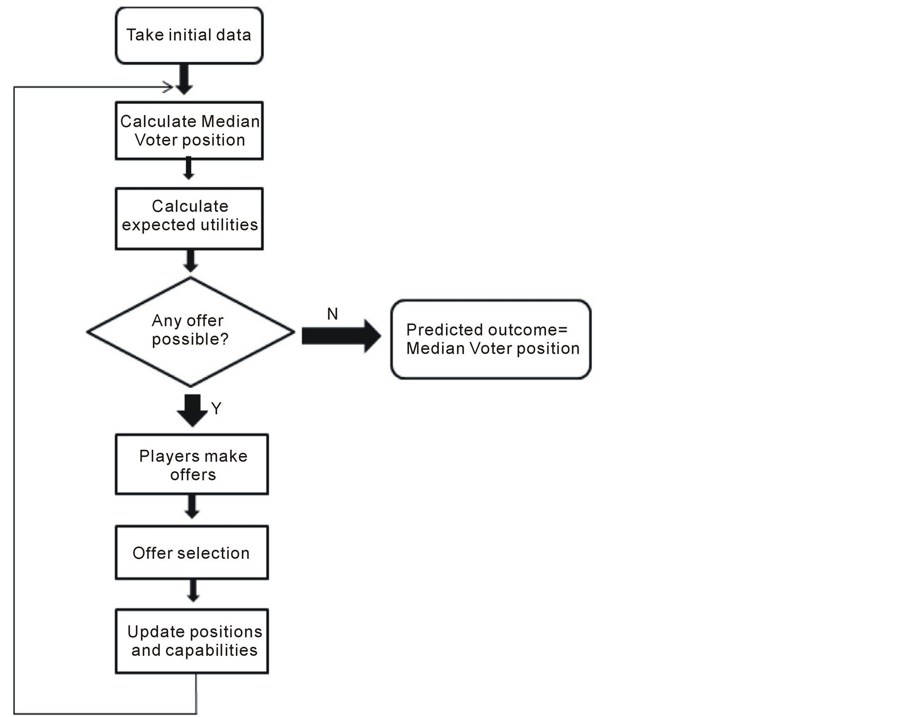
Figure 1. Main steps in Preana algorithm.
These arrays define players’ initial state. The most important array is the array of positions (x[]). Each player has an ideal position on a one-dimensional left to right continuum.The more two given players ideal outcomes conflict, the more their distance is on this scale. The unit of this position is specified for each given problem. Array of salience (s[]) determines the priority of the issue and how much importance it holds for each player. Array of capability (c[]) determines how much power or capability a player has on the issue. table 1 represents an example of these three arrays from [5] . This is an example about “What is the attitude of each stakeholder with regard to the floor price of oil in three months time at which Saudi production should decrease?”
2.2. Median Voter Position
The model focuses on the application of Black’s median voter theorem [6] and Banks’ theorem on the monotonicity between certain expectations and the escalation of political disputes [7] . The median voter theorem states that a majority rule voting system will select the outcome most preferred by the median voter [8] . The median voter position is the position of the player that, when compared with every other player, is preferred by more votes. In each round of negotiations, the player whose position is closest to the median voter position is the winner. This implies that the winner is the player who has more support from others. According to Bruce Beuno de Mesquita [5] , the votes for j versus k, are:
 (1)
(1)
The difference between the distance of player i’s position from that of player j and player k is calculated and normalized. This, multiplied by player i’s capability and salience, shows player i’s support for player j versus

Table 1 . Sample of the input.
player k which is
 in the equation. This support is calculated from all players. The sum of the support player j gets versus player k and every other player is the total support it can get at the associated round. The total support is calculated for all players and the one that has the maximum total support is the median voter position at that round.
2.3. Expected Utilities
In each round, players make challenge offers to other players aiming to make others shift their positions towards their ideal position. These offers are made based on the expected utilities calculated for each player versus the rest of the players. Players try to maximize their own pay off by making offers to players whom they think they can convince or force to make a coalition with. At the same time, players try to respond to the offer that leads to the maximum pay off for them or at least requires them to move the least from their ideal position. Figure 2 illustrates the sequence of plays [1] .
The expected utility of player(i) for challenging player(j) from player(i)’s point of view [9] can be calculated as:
 (2)
(2)
According to Figure 2,
 is the salience of the issue for player j,
 is the probability of success for player i,
 is the expected utility of success for player i,
 is the expected utility of losing for player i, Q is the probability of status quo,
 is the expected utility from remaining in stalemate, T is the probability that situation improves for player i when it does not challenge player j, and
 is the expected utility in this situation.
 is the expected utility in the situation that player i does not challenge player j, player j is challenged by others and the results of these challenges worsens the situation for player i.
 is the median voter position at each iteration.
Equation (2) is estimated from four perspectives [5] ;
(1) i’s expected utility for challenging j from i’s point of view
(2) j’s expected utility for challenging i from j’s point of view
(3) i’s expected utility for challenging j from j’s point of view
(4) j’s expected utility for challenging i from i’s point of view The calculation of ,
,
 ,
,
 ,
,
 and
and
 are explained in details in [3] , but here are the equations:
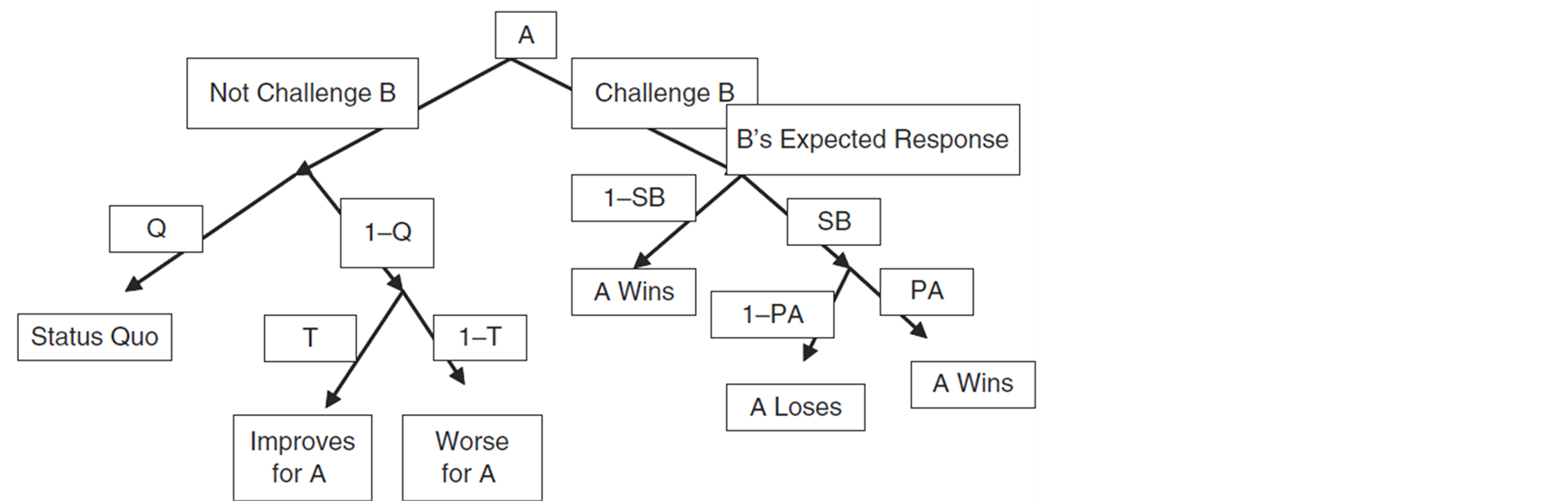
Figure 2. Game tree in expected utility model.


The above equations are used to calculate the expected utility of player i for challenging player j from i’s point of view.
 is the position of player i,
 is the position of player j,
 is the highest position in the game and
 is the lowest position in the game.
 is the risk component for player i versus player j.
When player i wants to make an offer to player j, it calculates its own expected utility from this challenge and compares it to what it perceives of Player j’s expected utility versus himself. We have concluded that:


And using ,
,
 ,
,
 ,
,
 and
and
 Player j’s expected utility versus player i, from player i’s point of view, is
 :
:
 (3)
(3)
2.4. Probability of Success (P)
The probability of success for player i in competition with player j is also calculated by the support of third-party players for player i’s policies versus player j’s policies. Similar to finding the median voter position, it is not only about which player’s policies the parties prefer, but also the third-parties’ salience on the issue and their capability or power are considered. Equation (4) shows the probability of success for player i in competition with player j according to Expected Utility Model [3] .
 (4)
(4)
where ,
,
 and
and
 are the positions for player i, player j and player k respectively.
 is the power of player k and
 is the salience and importance of the issue for player k.
The numerator calculates the expected level of support for i. The denominator calculates the sum of the support for i and for j so that the expression shows the probability of success for i, and it obviously falls in the range of 0 and 1.
2.5. Probability of Status Quo (Q)
The calculation of the probability of status quo (Q) has never been talked about in any of Bruce Beuno de Mesquita’s publications. He considers Q constant in some publications such as [9] in which he considers Q to be 1. This means that when i decides not to challenge j, i and j remain in stalemate with each other and the change in their positions in responding to other players’ offers does not affect their situation against each other. In different publications [10] and [11] , he considers Q to be 0.5 which means whether the change in the position affects players situations versus one another or not, is completely random. In this work, we have been able to calculate this probability for each pair of players. According to Figure 2, when A does not challenge B, B is challenged by other players and may lose and be forced to move. If B moves, its position changes and its distance to A either decreases (with probability T) or increases (with probability 1-T). Therefore, the probability of status quo in this situation is the probability that B does not move at all. This is the probability that B wins the challenge with every other player except A in that round. This probability is calculted as follows:

The probability that player(i) wins every challenge against another player(k), is the sum of two probabilities. first, the probability that player(i) challenges player(k) and player k does not challenge it back and surrenders which is . Second, the probability that player(i) challenges player(k) and player(k) does respond to its challenge and again player(i) wins this confrontation which is
 . The probability that player(i) wins against every other player except player(j), is the multiplication of this sum for all players except player(j).
2.6. Probability of Positive Change (T)
According to Figure 2, when A decides not to challenge B, but B moves due to other challenges, its move either improves or worsens the situation for A. B move would be towards the median voter position, so the positions of A, B and the median voter
 versus one another determines whether B moves closer to A or further away from it. If B moves closer to A, it improves the situation for A, so T = 1. If B moves further away from A, it worsens the situation for A, so T = 0 [3] .
2.7. Offer Selection
According to Bruce Beuno de Mesquita [5] , the probability with which confrontation, compromise or capitulation occur can be easily displayed in a polar coordinate space. This space is divided into six sections and the boundary between each two is considered to be a turning point in the probability functions. Figure 3 shows this polar coordinate space, along with associated labels for each of the six sections.
In Bruce Beuno de Mesquita publications, there is no exact definition of how these sectors are defined or separated from one another or how the players decide to whom they make a challenge offer and to whose offer they respond. However, he does explain how offers are made based on the expected utilities of a player versus another, combined with what the proposer perceives of the expected utility of the other player versus itself. In Preana, if the two players both assume they have the bigger utility compared to the opponent and that their utility is big enough to make the other player move to their position, they both make challenge offers to one another and they both stick to their offer and they confront. Clearly this has high cost for both players. If a player thinks it has bigger utility, but not big enough to make the other player completely move to its own position, he offers a compromise. If the other player responds to this offer, they both move towards each other. According to Bruce beuno de Mesquita, they move by weighted average of i’s and j’s expectations [5] . If a player receives an offer and knows that the proposer is too strong for it to challenge, it gives in and completely moves to the proposer’s position. If both players think there is no positive utility in challenging each another, they make no offer and stay in the stalemate zone.
The median voter position is calculated at the beginning of the first round of negotiation and is selected to be the winner position of the game with the initial positions, capabilities and salience. At the end of each round of negotiation, every player has a set of offers that has to choose from and then responds to the one that considers is the best choice to maximize its pay off. If such an offer does not exist, it chooses the offer that requires it to move the least from its ideal position [5] . After all players have selected the offer they want to respond to, they move to the position associated with the offer and the array of position and capability are updated. In the following round, the median voter position, the probabilities of success and status quo, the expected utilities and the risk factor are all calculated with the updated position array, and then new offers are made. The game continues until it reaches an equilibrium and that is when no player has an offer to make to the other players given every other players’ position. In this situation, all payers prefer to stay at their current position. The median voter at this final round would be the winning position. The player whose ideal position in the initial array of inputs is nearest to this median voter, is most likely to be able to enforce it’s ideal outcome.
3. Risk
In this section, we briefly define the Expected Utility Model’s risk taking component. This function calculates a risk or security value for each player in confrontation with all other players. In Preana, we add learning module
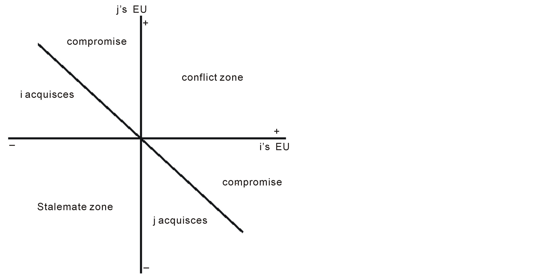
Figure 3. Scenarios in expected utility model.
to this function to model the brain of each player. The players learn from the offers they make in each round. When player(i) makes an offer to player(j), and does not result in a positive pay off, he concludes that it had underestimated player(j)’s abilities which means that next time it is more careful in confronting player(j). And on the other hand, when it can enforce an offer, has more confidence in confrontation with player(j) in the future.
3.1. Expected Utility Model’s Risk-Taking Component
Expected Utility Model’s risk taking component is explained in details in Bruce Beuno de Mesquita and Stokman [12] . The risk-taking component is a trade off between political satisfaction and policy satisfaction [13] . Political satisfaction or security is being seen as a member of winning coalition while policy satisfaction is supporting the policy that is most close to that of the player itself even if that policy does not win. The rate at which players make this trade-off is different from one another. The security of a player increases and the risk decreases by taking a position close to the median voter position. Therefore, the players who take positions close to the median voter position, who is the winner at the associated round, are feeling more vulnerable and tend to be more risk averse [5] . What enters the calculation of risk in the Expected Utility Model, is the actual expected utility, the maximum feasible expected utility and the minimum feasible expected utility. Algebraically, the risk-taking component is calculated as follows [9] :
 (5)
(5)
and
 (6)
(6)
As seen in Equation (3), the risk factor is used in the calculation of expected utilities, and according to Equation (5), risk is calculated using the expected utilities. It can be interpreted from Bruce Beuno de Mesquita’s statements that first the expected utilities are calculated without considering the risk (r = 1) and then these utilities are used to calculate the risk for each player [3] .
3.2. Preana’s Risk-Taking Component
According to Bruce Beuno de Mesquita [9] the purpose of equation (6) is that r[i] ranges between 0.5 and 2. However, according to this equation, the greater R[i], the smaller r[i]. So r[i] is actually the level of security rather than risk of player i. That explains why expected utilities are exponentially increasing by r which is a positive number between 0.5 and 2. This security level is calculated in each round taking into account the support each player gets from other players, the expected utilities, and the distance from the median voter position. What seems to be left out in the Expected Utility Model is that players cannot look ahead in rounds or even look back and learn from their mistakes or achievements. There are several rounds of negotiations before players reach an equilibrium and the game comes to an end. It is possible that player(i) underestimates player(j)’s capabilities and its supporters and makes a challenge offer and consecutively loses some utility. In reality, this should change player i’s assumptions about player j, and therefore, next time when i wants to make an offer to j, does it more conservatively. To monitor the offers and to learn from the outcomes, we have modeled the brain of each player. Bruce Beuno de Mesquita calculates r[i] for each player using the security for player(i) in confrontation with any other player. In contrast, we have extended the security to be a twodimensional array. R[i][j] is the risk of player i in confrontation with player j. The array is initialized with the risk calculated from the Expected Utility Model in each round and then adjusted in each round. We have taken the idea of including a learning matrix and a learning rate from the Q-learning method introduced by Watkins in 1989 [14] .
Here is how we form the learning matrix:
• Make a two-dimensional matrix named learn and initiate it to all 0• At the end of each round, each player monitors the offers it has made• If a proposal has been made by i and not responded to by j, decrement learn [i] [j] by 1• If a proposal has been made by i that leads to confrontation in which i has to move towards j, decrement learn [i] [j] by 3• If a proposal has been made by i that leads to compromise in which i has to move more than j, decrement learn [i] [j] by 2• If a proposal has been made by i that leads to i having to capitulate and move towards j, decrement learn [i] [j] by 3• If a proposal has been made by i that leads to confrontation in which j has to move towards i, increment learn [i] [j] by 1• If a proposal has been made by i that leads to compromise in which j has to move more than i, increment learn [i] [j] by 2• If a proposal has been made by i that leads to j having to capitulate and move to i, increment learn [i] [j] by 3.
As specified above, the learn matrix is updated after each round by considering each offer and its outcome for the proposer. If the outcome is positive, it increases the security player i feels to challenge player j next time. However, if the outcome is negative, player i learns that it had underestimated player j’s expected utility versus its own and its security level versus player j decreases. The more the number of the loss or gains is, the more effective is matrix learn.
Here is how we adjust the risk:
r[i][j]elements are initiated with r[i]of the Expected Utility Model. Then in each iteration:
 (7)
(7)
The security level is updated after each round and kept in the memory of each player for future rounds. Equation (7) indicates that the more importance or salience an issue has for a player, the less risk that player can afford on the issue. If a player is rather indifferent on the issue, the experience of a loss or an unseen opportunity will not be so heavy on it. The possibility of this player making the same mistake again is more than a player to whom the issue is of great priority and importance. That is why we do not consider the learning rate to be constant for each player as it is in Q-learning. The learning rate is a multiplication of salience and a constant .
.
In this article and the following case studies, we have considered
 to be set to 0.01. We have selected 0.01 experimentally given the fact that this value should be very small but not too small, so that it can make a difference. It should be small because the risk factor is in the range of 0.5 and 2 and if
 is too large, it will change the risk factor irrationally and might even push it out of range. Furthermore, if
 is too small, it does not make any difference in the outcome of the equations when added to the initial risk factor. Experimenting with different values of
 for the different problems in hand, we realized that different problems have different tolerance for the level of increase in
 before starting to respond irrationally. Finding the right way to calculate
 for a given problem domain would be a target for the future work.
4. Results
To evaluate the performance of Preana, we have included two case studies from Bruce Beuno de Mesquita’s publications. We have compared the results of Preana’s prediction to that of the Expected Utility Model and the real outcomes of the issue if available. There are hundreds of pages of output for each example that can be interpreted which include useful information such as the offers that are made in each round, the ones that can be enforced, the outcome of each confrontation in each round, formed coalitions or separations, and the flow of the whole system towards the final outcome. Here, for each case study, we only show the change in the position of each player and the median voter position over time (rounds).
4.1. Case Study 1: Predicting the Floor Price of Oil in Three Months Time
As our first case study, we consider the same example that its input data is shown in table 1. Figures 4-7 show the players’ positions and the winner position in subsequent rounds. As we see in figures 4-6, all of the players in this game change their positions over rounds until they all reach a position very close to the winning position which is 13.11. Figure 7 shows the Median voter or the winning position in different rounds of negotiations which ends up to be equal to 13.11 in the last round where equillibrium is reached.
Preana’s predicted price, as shown in Figure 6 and Table 2 is 13.11 which is closest to the ideal price for
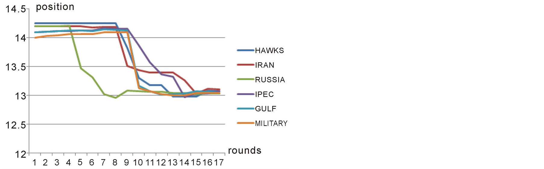
Figure 4. Position of first group of players over different rounds in case study 1.
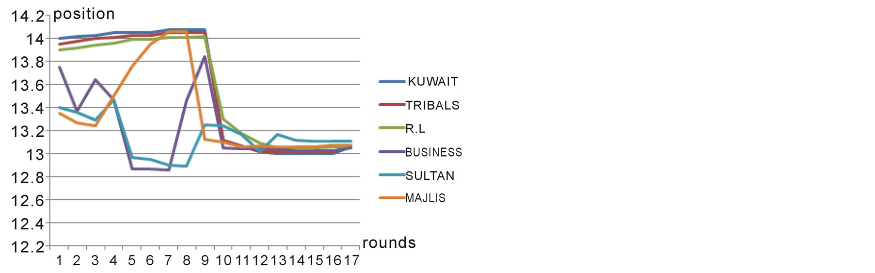
Figure 5. Position of second group of players over different rounds in case study 1.
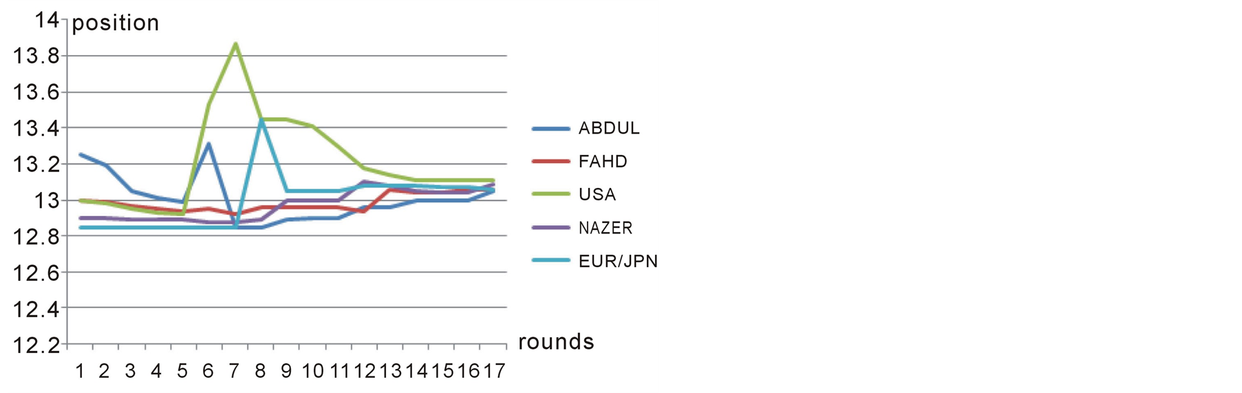
Figure 6. Position of third group of players over different rounds in case study 1.
USA and FAHD which is 13.00. Bruce Beuno de Mesquita [5] states that the outcome of the Expected Utility Model for this case study is 13.00 which is very close to what is reported by Preana.
4.2. Case Study 2: The Years of Introduction of Emission Standards for Medium Sized Automobiles
This is another case study from Bruce Beuno de Mesquita [12] . The issue is to predict the number of years that would need to pass before the introduction of emission standards for medium sized automobiles. The players and their initial capabilities, positions and salience are illustrated in table 3. Figures 8-10 show the players’ positions and the winner position in subsequent rounds.
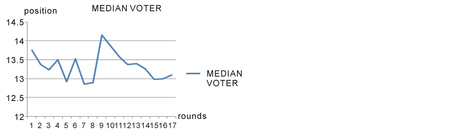
Figure 7. The median voter position in each round in case study 1.
Figure 8. Position of first group of players over different rounds in case study 2.
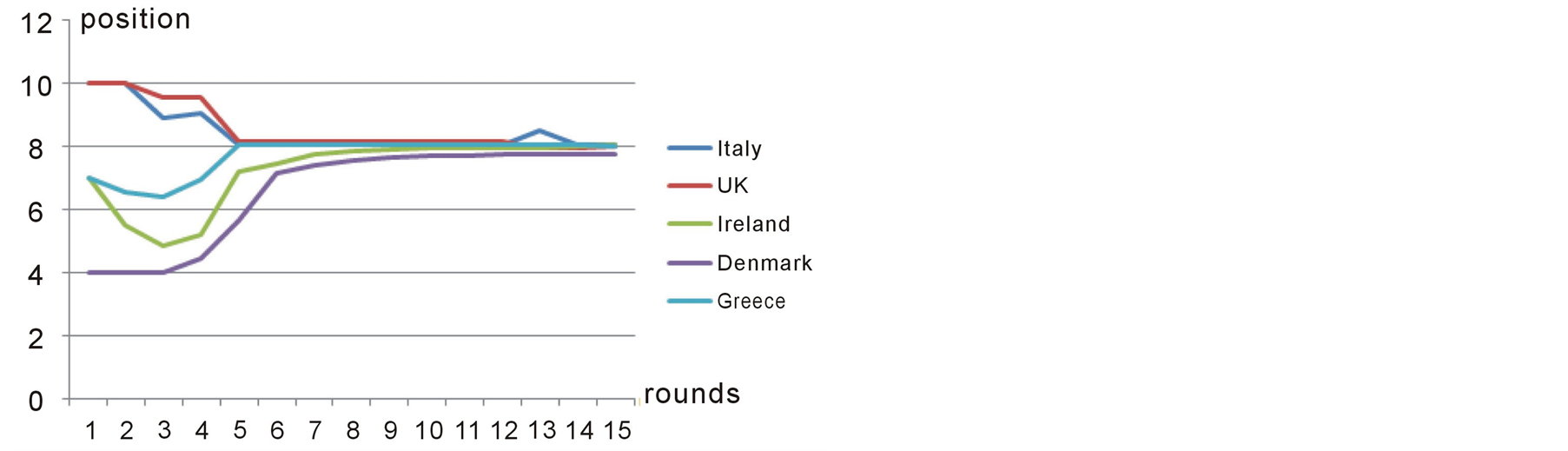
Figure 9. Position of second group of players over different rounds in case study 2.
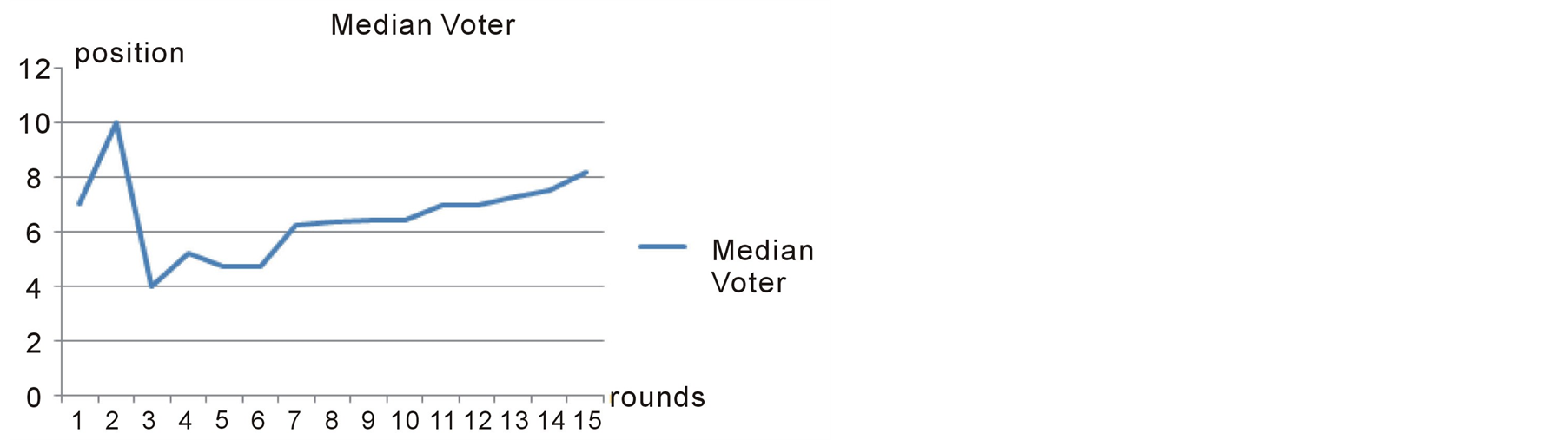
Figure 10. The Median voter position in each round in case study 2.
Table 2. Output for case study 1.
Table 3. Input for case study 2.
According to Bruce Beuno de Mesquita [12] , the outcome of the Expected Utility Model for this case study is 8.35 and the actual delay has been 8.83 years. As shown in figure 9, Preana predicts the outcome to be 8.15 years.
4.3. Case Study 3: The Winner of Iran’s 2013 Election
The last case study is the prediction of the recent 2013 presidential election in Iran. The input for Preana is taken from the web-poles before the election and interview with experts about the initial situation of each candidate before the election. The candidates’ positions are determined on a one-dimensional scale, the most reformist being on the position 10 and the most fundamentalist being on the position 1. The candidates and their initial capabilities, positions and salience month period before the election are shown in table 4. Figures 11-13 show the players’ positions and the winner position in subsequent rounds.
Preana shows the winner of the election to be position 9.2 which is in the middle of the ideal position for the two reformist candidates Aref and Ruhani. What happened in reality was exactly like what is shown in figure 12. Reformists got stronger and stronger during the debates and right before the election, Ruhani and Aref made a coalition together and Aref left the competition in favor of Ruhani. Eventually Ruhani won the election [15] . This is more clearly illustrated in Figure 13.
Table 4. Input for case study 3.
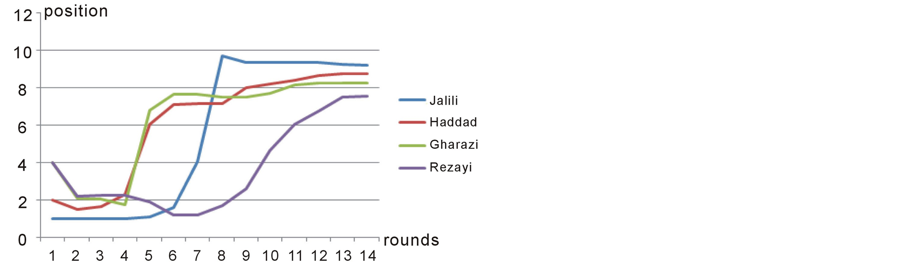
Figure 11. Position of first group of players over different rounds in case study 3.
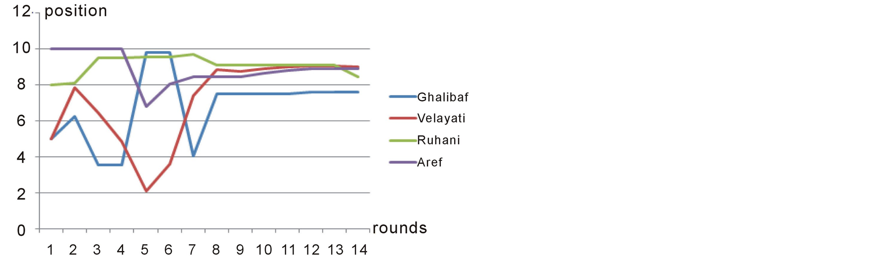
Figure 12. Position of second group of players over different rounds in case study 3.
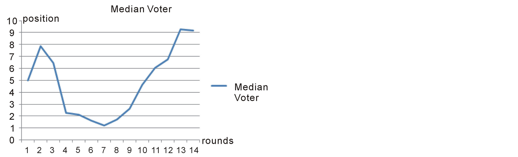
Figure 13. The median voter position in each round in case study 3.
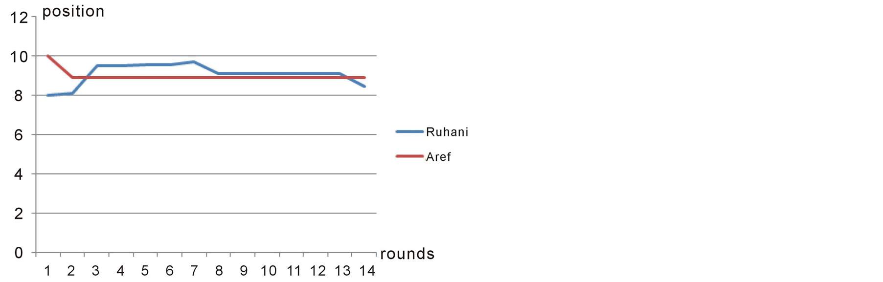
Figure 14. Aref and Ruhani’s coalition in case study 3.
5. Conclusion
This work was initiated with two major objectives in mind. The first objective was to uncover the hidden elements of today’s most promising game theory based predictive analysis tool developed by Bruce Bueno De Mesquita. On this front, we developed a methodology which produces comparable results to what Buenos model generates. The second objective was to improve what game theory can offer by applying machine learning to game theory. The authors believe both of these objectives are reached. Three case studies were presented and evaluated for the proof of concept. These case studies compared the results of the present work with the prior one. The third case study illustrated the power of this work in predicting real word political phenomena such as recent presidential election in Iran. We believe integration of game theory and machine learning is not only promising but even necessary to move towards more dynamic and realistic approaches. This work is just a stepping stone towards such integration.
References
- de Mesquita, B.B. (2011) A New Model for Predicting Policy Choices: Preliminary Tests. Conflict Management and Peace Science, 28, 65-87. http://dx.doi.org/10.1177/0738894210388127
- Feder, S.A. (1995) FACTIONS and Policon: New Ways to Analyze Politics. In: Westerfield, H.B. (Ed.), Inside CIA’s Private World: Declassified Articles from the Agency’s Internal Journal, Yale University Press, Yale, CT, 274-292.
- Scholz, J.B., Calbert, G.J. and Smith, G.A. (2011) Unravelling Bueno De Mesquita’s Group Decision Model. Journal of Theoretical Politics, 23, 510-531. http://dx.doi.org/10.1177/0951629811418142
- Ueng, B. (2012) Applying Bruce Bueno de Mesquita’s Group Decision Model to Taiwan’s Political Status: A Simplified Model. The Visible Hand: A Cornell Economics Society Publication, Ithaca, NY.
- de Mesquita, B.B. (1997) A Decision Making Model: Its Structure and Form. International Interactions: Empirical and Theoretical Research in International Relations, 23, 235-266. http://dx.doi.org/10.1080/03050629708434909
- Black, D. (1948) On the Rationale of Group Decision-Making. Journal of Political Economy, 56, 23-34. http://dx.doi.org/10.1086/256633
- Banks, J.S. (1990) Equilibrium Behavior in Crisis Bargaining Games. American Journal of Political Science, 34, 599-614. http://dx.doi.org/10.2307/2111390
- Holcombe, R.G. (2006) Public Sector Economics. Pearson Prentice Hall, Upper Saddle River, 155.
- De Mesquita, B.B. (1985) The War Trap Revisited: A Revised Expected Utility Model. American Political Science Review, 79, 156-177.
- De Mesquita, B.B. and Lalman, D. (1986) Reason and War. American Political Science Review, 80, 1113-1129.
- De Mesquita, B.B. (2009) A New Model for Predicting Policy Choices: Preliminary Tests. 50th Meeting of the International Studies Association, New York, 15-18 February 2009, 36p.
- De Mesquita, B.B. (1994) Political Forecasting: An Expected Utility Method. In: Stockman, F., Ed., European Community Decision Making, Yale University Press, Yale, Chapter 4, 71-104.
- Lamborn, A. (1991) The Price of Power. Unwin Hyman, Boston.
- Watkins, C.J.C.H. (1989) Learning from Delayed Rewards. PhD Thesis, University of Cambridge, England.
- Hassan Rouhani Wins Iran Presidential Election BBC News, 15 June 2013. http://www.bbc.com/news/world-middle-east-22916174
NOTES

*Corresponding author.