Natural Science
Vol.4 No.12(2012), Article ID:25372,9 pages DOI:10.4236/ns.2012.412127
Approximate analytical solution of non-linear reaction diffusion equation in fluidized bed biofilm reactor
![]()
Department of Mathematics, The Madura College, Madurai, India; *Corresponding Author: raj_sms@rediffmail.com
Received 13 October 2012; revised 12 November 2012; accepted 27 November 2012
Keywords: Fluidized Bed Biofilm Reactor; Non-Linear Reaction Diffusion Equation; Phenol; Effectiveness Factor; Modified Adomian Decomposition Method
ABSTRACT
A mathematical model for the fluidized bed biofilm reactor (FBBR) is discussed. An approximate analytical solution of concentration of phenol is obtained using modified Adomian decomposition method (MADM). The main objective is to propose an analytical method of solution, which do not require small parameters and avoid linearization and physically unrealistic assumptions. Theoretical results obtained can be used to predict the biofilm density of a single bioparticle. Satisfactory agreement is obtained in the comparison of approximate analytical solution and numerical simulation.
1. INTRODUCTION
There has been much interest in the development of biofilms. Biofilms play significant roles in many natural and engineered systems. The importance of biofilms has steadily emerged since their first scientific description in 1936 [1]. Mechanistically based modeling of biofilms began in the 1970s. The early efforts focused mainly on substrate flux from the bulk liquid into the biofilm. Biofilms have been used to treat wastewater since the end of the 19th century. Biofilm reactors with larger specific surface areas were developed starting in the 1980s [2-4]. Biofilm modeling was advanced by Rittmann and McCarty [5,6], who based their models on diffusion (Fick’s law) and biological reaction (Monod kinetics) within the biofilm and liquid-layer mass transfer from the bulk liquid. The mathematical model to describe the oxygen utilization for a TFBBR in wastewater treatment was developed by Choi [7], which was proposed to describe the oxygen concentration distribution. This model consisted of the biofilm model that described the oxygen uptake rate and the hydraulic model that presented characteristics of liquid and gas phase [8].
The fluidized bed reactor (FBB) is the reactor which carries on the mass transfer or heat transfer operation using the fluidization concept. At first it was mainly used in the chemical synthesis and the petrochemistry industry. Because this kind of reactor displayed in many aspects its unique superiority, its application scope was enlarged gradually to metal smelting, air purification and many other fields. Since 1970’s, people have successfully applied the fluidization technology to the wastewater biochemical process field. An FBB is capable of achieving treatment in low retention time because of the high biomass concentrations that can be achieved. A bioreactor has been successfully applied to an aerobic biological treatment of industrial and domestic wastewaters. An FBB offers distinct mechanical advantages, which allow small and high surface area media to be used for biomass growth [9-12].
Fluidization overcomes operating problems such as bed clogging and the high-pressure drop, which would occur if small and high surface area media were employed in packed-bed operation. Rather than clog with new biomass growth, the fluidized bed simply expands. Thus for a comparable treatment efficiency, the required bioreactor volume is greatly reduced. A further advantage is the possible elimination of the secondary clarifier, although this must be weighed against the mediumbiomass separator [10-12].
Abdurrahman Tanyolac and Haluk Beyenal proposed to evaluate average biofilm density of a spherical bioparticle in a differential fluidized bed system [13]. To our knowledge, no general analytical expressions for the concentration of phenol and effectiveness factor have been reported for all values of the parameters λ, α and f. However, in general, analytical solutions of non-linear differential equations are more interesting and useful their numerical solutions, as they are used to various kinds data analysis. Therefore, herein, we employ analytical method to evaluate the phenol concentration and effectiveness factor for all possible values of parameters.
2. MATHEMATICAL FORMULATION OF THE PROBLEM
The details of the model adopted have been fully described in Haulk Beyenal and Abdurrahman Tanyolac [14]. Figure 1 represents a general kinetic scheme of differential fluidized bed biofilm reactor (DFBBR).
1. Base storage; 2. Heating strip; 3. Trap; 4 & 5. Sponge plug; 6. Dissolved oxygen electrode; 7. Combined gas feed; 8. Temperature control unit; 9. Thermocouple; 10. Thermometer; 11. Pulse dampener; 12. Steel screen; 13. Non-fluidized medium (river sand); 14. Air bubbles; 15. Support particle (active carbon; 16. Biofilm; 17. Acid storage; 18. Air sparger; 19. Oxygenerator; 20. Differential fluidized bed biofilm reactor (DFBBR); 21. pH electrode; AT—air trap; FCF—fresh culture feed (only for start up); GCV—gas flow control valve; GFM—gas flow meter; P1—pump for fresh feed; P2—fluidized bed combined feed pump; P3—pump for base; P4—pump for acid; R-rotameter; DOM—dissolved oxygen meter; pHM —pH meter; pHC—pH controller; TC—temperature controller; TM—temperature measurement; VC—voltage control.
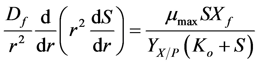
The biological reaction is described by the Monod relationship, which is a nonlinear expression. The differential equation for diffusion with Monod reaction within
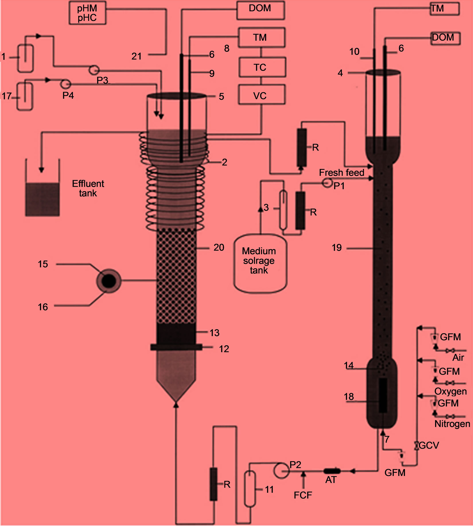
Figure 1. A schematic diagram of differential fluidized bed biofilm reactor (DFBBR) system [14].
the biofilm is [13]
 (1)
(1)
where S is the phenol concentration,  is the maximum specific growth rate of substrate,
  is the average effective diffusion coefficient of the limiting sub strate,
  is the average biofilm density,
  is the yield coefficient for phenol, and
  is the half rate kinetic constant for phenol. The equation can be solved subject to the following boundary conditions [13]:
 (2)
(2)
 (3)
(3)
where  denotes biofilm surface substrate concentration, r is the radial distance, rp is the radius of clean particle, and rb is the radius of biofilm covered bioparticle. The effectiveness factor for a spherical bioparticle is
 (4)
(4)
Normalized Form
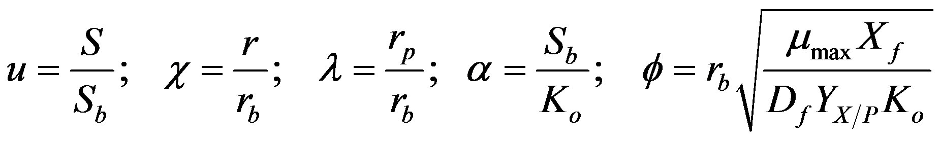
The above differential equation (Eq.1) for the model can be simplified by defining the following normalized variables,
 (5)
(5)
where  represent normalized concentration, distance and radius parameters, respectively. α denotes a saturation parameter and f is the Thiele modulus. Furthermore, the saturation parameter α describes the ratio of the phenol concentration within the biofilm
  to the rate kinetic constant for phenol
 . Then Eq.1 reduces to the following normalized form
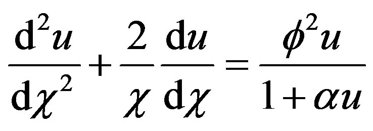 (6)
(6)
The boundary conditions reduce to
 (7)
(7)
 (8)
(8)
The effectiveness factor in normalized form is as follows:
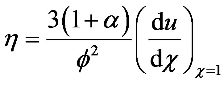 (9)
(9)
3. ANALYTICAL EXPRESSION OF CONCENTRATION OF PHENOL USING MODIFIED ADOMIAN DECOMPOSITION METHOD (MADM)
MADM [15-17] is a powerful analytic technique for solving the strongly nonlinear problems. This MADM yields, without linearization, perturbation, transformation or discretisation, an analytical solution in terms of a rapidly convergent infinite power series with easily computable terms. The decomposition method is simple and easy to use and produces reliable results with few iteration used. The results show that the rate of convergence of Modified Adomian decomposition method is higher than standard Adomian decomposition method [18-22]. Using MADM method, we can obtain the concentration of phenol (see Appendices A & B) as follows:
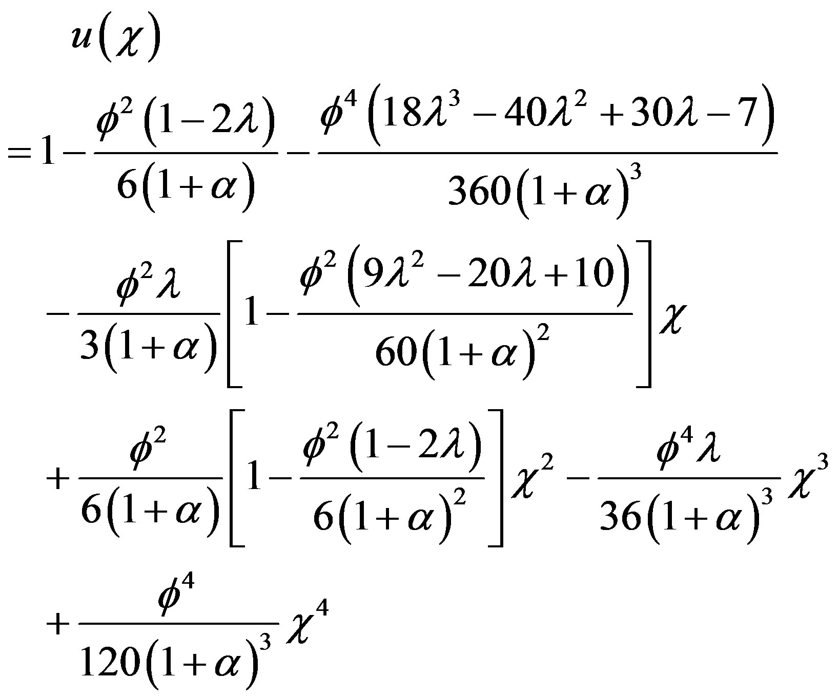 (10)
(10)
provided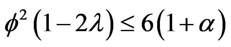 . Using Eq.9, we can obtain the simple approximate expression of effectiveness factor as follows:
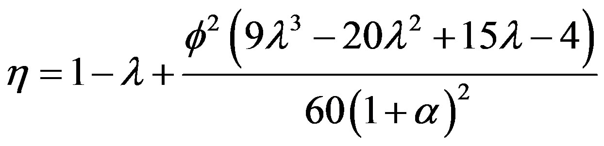 (11)
(11)
From Eq.11, we see that the effectiveness factor is a function of the Thiele modulus f, the saturation parameter α and the radius parameter λ. This Eq.11 is valid only when
 .
.
4. NUMERICAL SIMULATION
The non-linear equation [Eq.1] for the boundary conditions [Eqs.7 and 8] are solved by numerically. The function pdex4 in Scilab/Matlab software is used to solve the initial-boundary value problems for parabolic-elliptic partial differential equations numerically. The Scilab/ Matlab program is also given in Appendix C. Its numerical solution is compared with the analytical results obtained using MADM method.
5. RESULTS AND DISCUSSION
Eq.10 is the new, simple and approximate analytical expression of the concentration of phenol. Concentration of phenol depends upon the following three parameters , α and f. Figures 2(a)-(d) represent a series of normalized phenol concentration for the different values of the Thiele modulus. In this Figure 2, the concentration of phenol decreases with the increasing values of the Thiele modulus f. Moreover, the phenol concentration tends to one as the Thiele modulus f ≤ 0.1. Upon careful evaluation of these figures, it is evident that there is a simultaneous increase in the values of concentration of phenol u when f decreases. Furthermore, the phenol concentration increases slowly and rises suddenly when the normalized radial distance
 . Figure 3 represents the effecttiveness factor η versus normalized Thiele modulus f for different values of normalized saturation parameter α. From this figure, it is inferred that, a constant value of normalized saturation parameter α, the effectiveness factor decreases quite rapidly as the Thiele modulus f increases. Moreover, it is also well known that, a constant value of normalized Thiele modulus f, the effectiveness factor increases with increasing values of α.
The normalized effectiveness factor η versus normalized saturation parameter α is plotted in Figure 4. The effectiveness factor η is equal to one (steady state value)
 (a)
(a)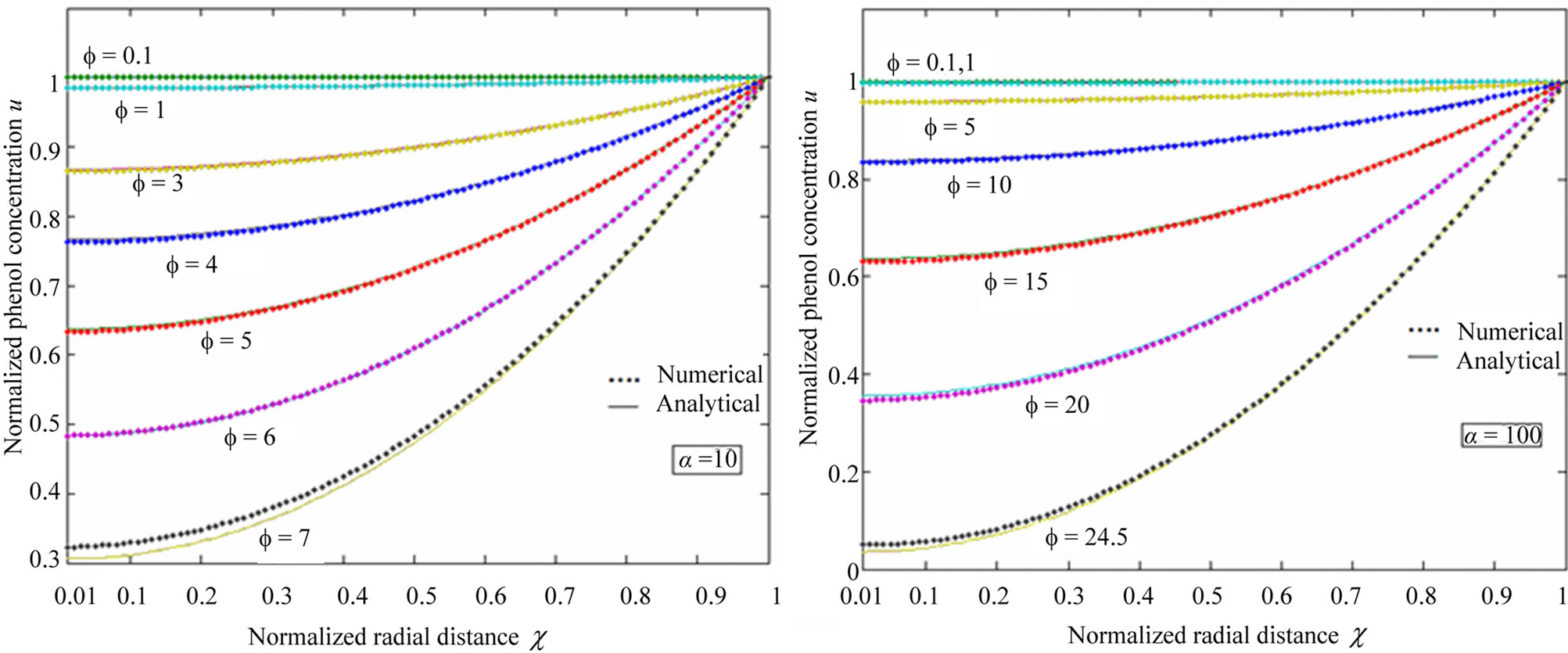 (b)
(b)
Figure 2. Plot of normalized phenol concentration u as a function of 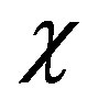 in fluidized bed biofilm reactor. The concentration were computed for various values of the Thiele modulus f and the radius parameter λ = 0.01 using Eq.10 when the normalized saturation parameter (a) α = 0.1; (b) α = 1; (c) α = 10; and (d) α = 100.
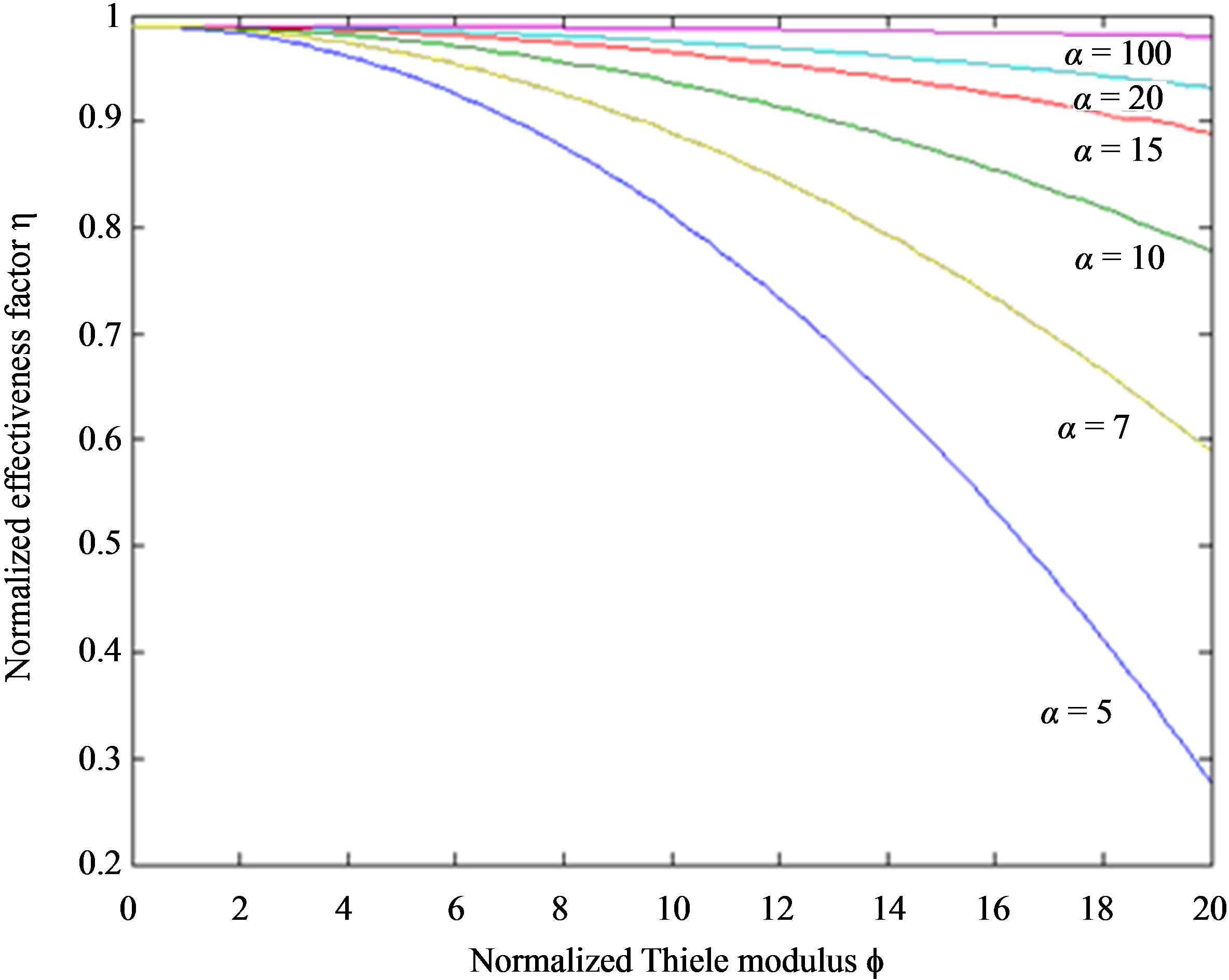
Figure 3. Plot of the normalized effectiveness factor η versus the Thiele modulus f. The effectiveness factor η were computed using Eq.11 for various values of the normalized saturation parameter α when the normalized radius parameter λ = 0.01.
Figure 4. Plot of the normalized effectiveness factor η versus normalized saturation parameter α. The effectiveness factor η were computed using Eq.11 for different values of the Thiele modulus f when the normalized radius parameter λ = 0.01.
when  and all values of f. Also the effectiveness factor η is uniform when
  and for all values of α. From this figure, it is concluded that the effectiveness factor decreases when f increases at x = 0. A three dimensional effectiveness factor η computed using Eq.11 for
  as shown in Figure 5. In this Figure 5, we notice that the effectiveness factor tends to one as the Thiele modulus decreases.
6. CONCLUSIONS
We have developed a comprehensive analytical formalism to understand and predict the behavior of fluidized bed biofilm reactor. We have presented analytical expression corresponding to the concentration of phenol in terms of  using the modified Adomian decomposition method. The approximate solution is used

Figure 5. Plot of the three-dimensional effectiveness factor η against f and λ, calculated using Eq.11 for α = 100.
to estimate the effectiveness factor of this kind of systems. The analytical results will be useful for the determination of the biofilm density in this differential fluidized bed biofilm reactor. The theoretical results obtained can be used for the optimization of the performance of the differential fluidized bed biofilm reactor. Also the theoretical model described here can be used to obtain the parameters required to improve the design of the differential fluidized bed biofilm reactor.
7. ACKNOWLEDGEMENTS
This work was supported by the Council of Scientific and Industrial Research (CSIR No.: 01(2442)/10/EMR-II), Government of India. The authors also thank the Secretary, The Madura College Board, and the Principal, The Madura College, Madurai, Tamilnadu, India for their constant encouragement.
REFERENCES
- Zobell, C.E. and Anderson, D.Q. (1936) Observationson the multiplication of bacteria in different volumes of stored sea water and the influence of oxygen tension and solid surfaces. Biological Bulletin, 71, 324-342. doi:10.2307/1537438
- Williamson, K. and McCarty, P.L. (1976) A model of substrate utilization by bacterial films. Journal of the Water Pollution Control Federation, 48, 9-24.
- Harremoës, P. (1976) The significance of pore diffusion to filter denitrification. Journal of the Water Pollution Control Federation, 48, 377-388.
- Rittmann, B.E. and McCarty, P.L. (1980) Model of steadystate-biofilm kinetics. Biotechnology and Bioengineering, 22, 2343-2357. doi:10.1002/bit.260221110
- Rittmann, B.E. and McCarty, P.L. (1981) Substrate flux into biofilms of any thickness. Journal of Environmental Engineering, 107, 831-849.
- Rittman, B.E. and McCarty, P.L. (1978) Variable-order model of bacterial-film kinetics. American Society of Civil Engineers. Environmental Engineering Division, 104, 889-900.
- Choi, J.W., Min, J., Lee, W.H. and Lee, S.B. (1999) Mathematical model of a three-phase fluidized bed biofilm reactor in wastewater treatment. Biotechnology and Bioprocess Engineering, 4, 51-58. doi:10.1007/BF02931914
- Meikap, B.C. and Roy, G.K. (1995) Recent advances in biochemical reactors for treatment of wastewater. International Journal of Environmental Protection, 15, 44-49.
- Vinod, A.V. and Reddy, G.V. (2003) Dynamic behaviour of a fluidised bed bioreactor treating waste water. Indian Chemical Engineer Section A, 45, 20-27.
- Sokol, W. (2003) Treatment of refinery wastewater in a three-phase fluidized bed bioreactor with a low-density biomass support. Biochemical Engineering Journal, 15, 1-10. doi:10.1016/S1369-703X(02)00174-2
- Gonzalez, G., Herrera, M.G., Garcia, M.T. and Pena, M.M. (2001) Biodegradation of phenol in a continuous process: Comparative study of stirred tank and fluidized-bed bioreactors. Bioresource Technology, 76, 245-251. doi:10.1016/S0960-8524(00)00092-4
- Sokol, W. and Korpal, W. (2004) Determination of the optimal operational parameters for a three-phase fluidised bed bioreactor with a light biomass support when used intreatment of phenolic wastewaters. Biochemical Engineering Journal, 20, 49-56. doi:10.1016/j.bej.2004.02.009
- Tanyolac, A. and Beyenal, H. (1996) Predicting average biofilm density of a fully active spherical bioparticle. Journal of Biotechnology, 52, 39-49. doi:10.1016/S0168-1656(96)01624-0
- Beyenal, H. and Tanyolac, A. (1998) The effects of biofilm characteristics on the external mass transfercoefficient in a fluidized bed biofilm reactor. Biochemical Engineering Journal, 1, 53-61. doi:10.1016/S1369-703X(97)00010-7
- Adomian, G. (1976) Nonlinear stochastic differential equations. Journal of Mathematical Analysis and Applications, 55, 441-452. doi:10.1016/0022-247X(76)90174-8
- Adomian, G. and Adomian, G.E. (1984) A global method for solution of complex systems. Mathematical Model, 5, 521-568. doi:10.1016/0270-0255(84)90004-6
- Adomian, G. (1994) Solving frontier problems of physics: The decomposition method. Kluwer Academic Publishers, Boston, 1994.
- Hasan, Y.Q. and Zhu, L.M. (2008) Modified adomian decomposition method for singular initial value problems in the second-order ordinary differential equations. Surveys in Mathematics and Its Applications, 3, 183-193.
- Hosseini, M.M. (2006) Adomian decomposition method with Chebyshev polynomials. Applied Mathematics and Computation, 175, 1685-1693. doi:10.1016/j.amc.2005.09.014
- Wazwaz, A.M. (1999) A reliable modifications of Adomian decomposition method. Applied Mathematics and Computation, 102, 77-86. doi:10.1016/S0096-3003(98)10024-3
- Wazwaz, A.M. (1999) Analytical approximations and Pade approximants for Volterra’s population model. Applied Mathematics and Computation, 100, 13-25. doi:10.1016/S0096-3003(98)00018-6
- Wazwaz, A.M. (2002) A new method for solving singular initial value problems in the second-order ordinary differential equations. Applied Mathematics and Computation, 128, 45-57. doi:10.1016/S0096-3003(01)00021-2
APPENDIX A
Basic Concept of the Modified Adomian Decomposition Method (MADM)
Consider the nonlinear differential equation in the form
 (A1)
(A1)
with initial condition
 (A2)
(A2)
where  is a real function,
  is the given function and A and B are constants. We propose the new differential operator, as below
 (A3)
(A3)
So, the problem (A1) can be written as,
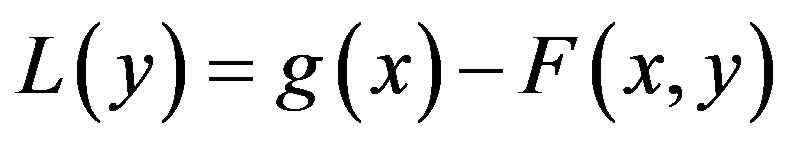 (A4)
(A4)
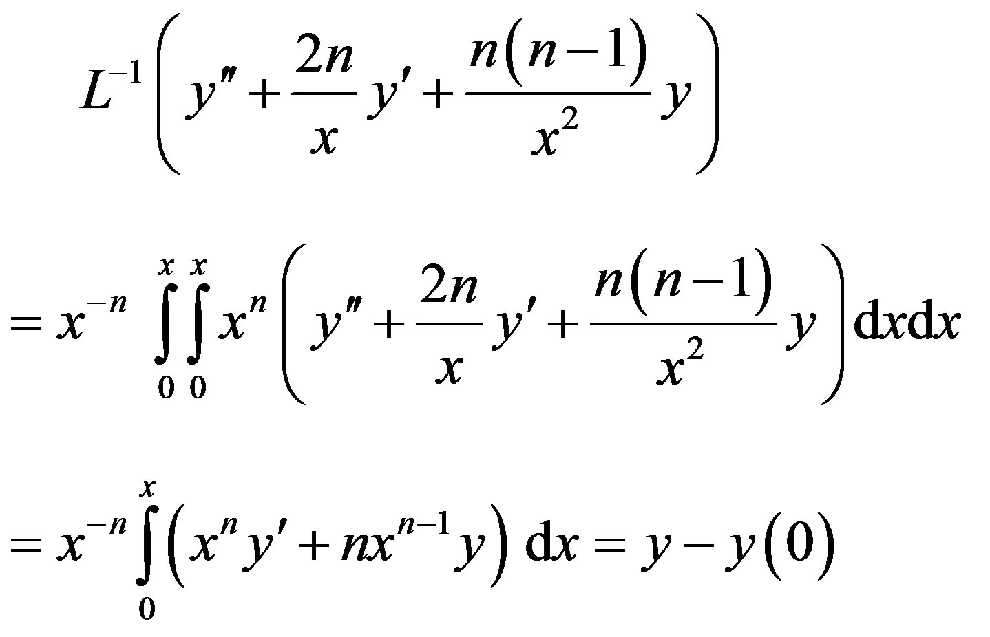
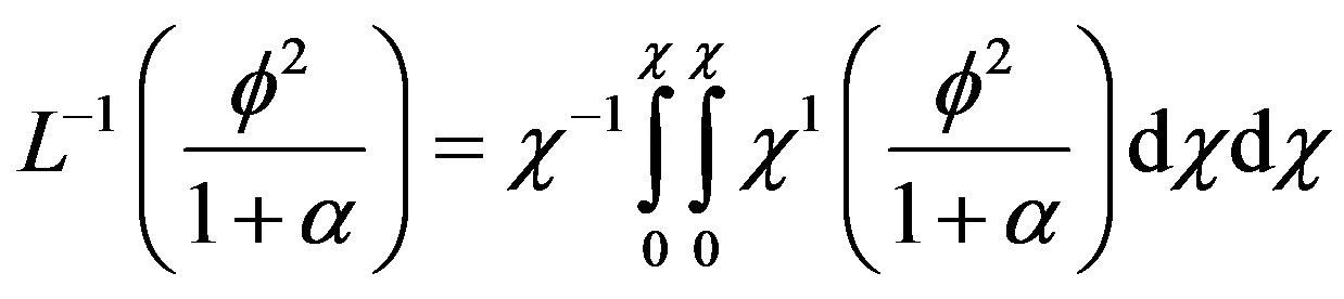
The inverse operator  is therefore considered a two-fold integral operator, as below.
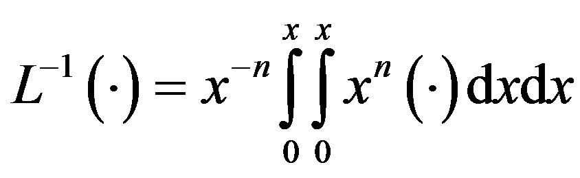 (A5)
(A5)
Applying  of (A4) to the first three terms
of Eq.A1, we find
By operating  on (A4), we have
 (A6)
(A6)
The Adomian decomposition method introduce the solution  and the nonlinear function
  by infinity series
 (A7)
(A7)
and
 (A8)
(A8)
where the components  of the solution
  will be determined recurrently and the Adomian polynomials An of
  are evaluated [23-25] using the formula
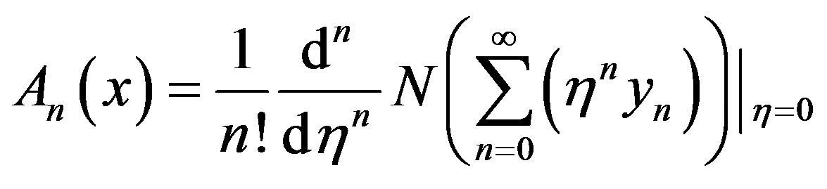 (A9)
(A9)
By substituting (A7) and (A8) into (A6),
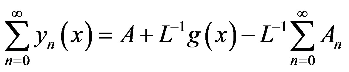 (A10)
(A10)
Through using Adomian decomposition method, the components  can be determined as
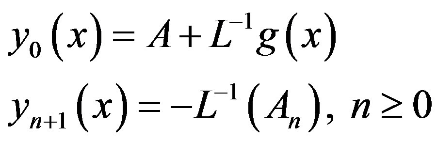 (A11)
(A11)
which gives
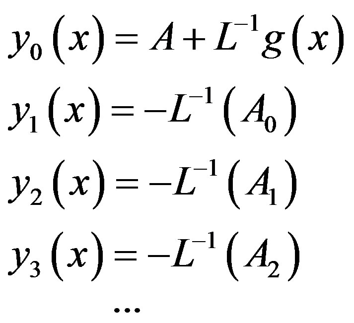 (A12)
(A12)
From (A9) and (A10), we can determine the components , and hence the series solution of
  in (A7) can be immediately obtained.
APPENDIX B
Analytical Expression of Concentration of Phenol Using the Modified Adomian Decomposition Method
In this appendix, we derive the general solution of nonlinear Eq.7 by using Adomian decomposition method. We write the Eq.7 in the operator form,
 (B1)
(B1)
where  .
.
Applying the inverse operator  on both sides of Eq.B.1 yields
 (B2)
(B2)
where A and B are the constants of integration. We let,
 (B3)
(B3)
 (B.4)
(B.4)
where
 (B.5)
(B.5)
Now Eq.B.2 becomes
 (B.6)
(B.6)
We identify the zeroth component as
 (B.7)
(B.7)
and the remaining components as the recurrence relation
 (B.8)
(B.8)
We can find An as follows:
 (B.9)
(B.9)
The initial approximations (boundary conditions Eqs.7 and 8 are as follows
 (B.10)
 (B.11)
and
 (B.12)
 (B.13)
Solving the Eq.B.7 and using the boundary conditions Eqs.B.10 and B.11, we get
 (B.14)
Now substituting n = 0 in Eqs.B.8 and B.9, we can obtain
 (B.15)
and  (B.16)
By operating  on (B.16),
 (B.17)
Now Eq.B.15 becomes
 (B.18)
Solving the Eq.B.18 and using the boundary conditions Eqs.B.12 and B.13, we get
 (B.19)
Similarly we can get
 (B.20)
Adding Eqs.B.14, B.19 and B.20, we get Eq.11 in the text.
APPENDIX C
Scilab/Matlab Program to Find the Numerical Solution of Eq.8 Is as Follows
function pdex1 m = 2;
x = linspace(0.01,1);
t = linspace(0,1000);
sol = pdepe(m,@pdex1pde,@pdex1ic,@pdex1bc,x,t);
u = sol(:,:,1);
figure plot(x,u(end,:))
title(‘u(x,t)’)
% -------------------------------------------------------------
function [c,f,s] = pdex4pde(x,t,u,DuDx)
c = 1;
f = DuDx;
phi=24.5;
alpha=100;
s =-(phi^2*u)/(1+alpha*u);
% -------------------------------------------------------------
function u0 = pdex1ic(x)
u0 = 1;
% -------------------------------------------------------------
function [pl,ql,pr,qr] = pdex4bc(xl,ul,xr,ur,t)
pl = 0;
ql = 1;
pr = ur-1;
qr = 0;