Engineering
Vol. 5 No. 4 (2013) , Article ID: 30494 , 7 pages DOI:10.4236/eng.2013.54046
Inexpensive Pipelines Health Evaluation Techniques Based on Resonance Determination, Numerical Simulation and Experimental Testing
School of Engineering, Manchester Metropolitan University, Manchester, UK
Email: wsabushanab@gmail.com
Copyright © 2013 Waheed Sami Abushanab. This is an open access article distributed under the Creative Commons Attribution License, which permits unrestricted use, distribution, and reproduction in any medium, provided the original work is properly cited.
Received February 19, 2013; revised March 20, 2013; accepted March 27, 2013
Keywords: Vibration Analysis’s; Condition Monitoring; ABAQUS CAE
ABSTRACT
In this paper, a non-destructive, reliable, and inexpensive vibration-based technique for evaluating Carbon steel pipes structure integrity. The proposed techniques allow a quick assessment of pipes structures at final pipe manufacturing stages and/or just before installation. A finite element modelling (FEM) using ABAQUS software was developed to determine the resonance mode of healthy Carbon steel pipe and a series of experiments were conducted to verify the outcomes of the modelling work. Consequently, the effects of quantified seeded faults, i.e., a 1 mm, 2 mm, 3 mm, and 4 mm diameter holes in the pipe wall on these resonance modes were determined using modelling work. A number of common used vibration analysis techniques were applied to detect and to evaluate the severity of those quantified faults. The amplitudes and frequencies of vibration signals were measured and compared. There were found to be in good agreement with the modelling work and provide important information on pipe construction condition and fault severity.
1. Introduction
The Maintenance of pipelines is of a great concern for oil companies. A proper and sensitive pipeline condition monitoring is desirable to predict leakage and other failure modes e.g. flaws, cracks, etc. Since pipeline passes through varied terrain, its condition will vary accordingly and inspecting the entire pipeline, using a specific methodology or tool, may not detect problems over its entire length. Most of the recent damage detection methods are relies on visual inspection or on localized measurements. Therefore, required that the vicinity of the damage is known a priori and that the portion of the structure being inspected is readily accessible thus subjected to these limitations, these experimental methods can detect damage on or near the surface of the structure.
Current damage detection methods are either visual or l Current damage detection methods are either visual or localized experimental methods, such as acoustic or ultrasound methods, magnetic field methods, radiography, eddy-current methods and thermal field methods. The diagnosis of damage in structural systems requires the identification of the location and type of damage and the quantification of the degree of damage.
Hu, Zhang and Liang [1] study case shows “small leak sensitive characteristics are recognized and the negative pressure wave inflexions are extracted by harmonic wavelet analysis, expressed in terms of harmonic wavelet time-frequency mesh map, time-frequency contour map”. Also, comparison was made between leak detection results of harmonic wavelet and Daubechies wavelet, and it was found that harmonic wavelet based small leak detection approach performed better. Sinha [2] used Lamb wave propagation in the wall of a pipe generated in a standoff manner for defect detection and found that this approach is accurate measurement of wall thickness on all kinds of materials and size only at the point of physical contact and not along the circumference of the pipe. Khulief, Khalifa, Ben Mansour and Habib [3] presented an experimental investigation to address the feasibility and potential of in pipe acoustic measurements for detection. They constructed a test rig for simulation purpose. It used to simulate a water transmission pipeline and permit different leak siaes, pressure and flow rates. They stated that the feasibility and limitations of invoking in-pipe measurements for leak detection were addressed. Hao, Yang, Shijiu and Zhoumo [4] proposed the principle of the distributed optical fiber pipeline leakage detecting and pre-warning system and the method to eliminate the desensitization. Moreover, they established the optical polarization model of oil and gas pipeline fiber warning system to analysis the desensitization that considered as a common problem of the fiber optic sensor. They stated that the experiment that the solution can solve the problem preferably and improve the locating accuracy and the sensitivity of the system. Jin, Yume and Ping [5] proposed new feature extraction and leak identification method to identify leaking in the presence of non-leak acoustic sources using autocorrelation analysis and approximate entropy algorithm. Moreover, they stated that a new method based on neural-network has been developed.
It is known from dynamic systems that a structure temporarily excited by an external force will vibrate at a frequency defined as the natural frequency. The natural frequency is characteristic of the entire structure and its boundary conditions. An external excitation applied to the structure at the same frequency as the structure’s natural frequency will result in resonance. At resonance, the structure will vibrate at higher than normal amplitude levels. Depending upon the overall system design, the amplitude of vibration at resonance can cause unwanted operating conditions as well as a catastrophic failure. Determining the structure’s natural frequency and maintaining the overall system at an operating condition that will not induce resonance can avoid this type of system failure. The natural frequencies of a structure can be determined by measuring frequency response. One means of measuring the frequency response is to impact test the structure. Impact testing is a measurement of the ratio of the structure’s transient response to the excitation impulse versus frequency.
2. Modal Dynamic Analysis
The modal dynamic procedure provides a time-history analysis of linear systems. The excitation is given as a function of time, and it is assumed that the amplitude curve is specified so that the magnitude of the excitation varies linearly within each increment. When the model is projected onto the Eigen modes used for its dynamic representation, we obtain the following set of equations at time t:
 (1)
(1)
where the ![]() and
and  indices span the Eigen space;
  is the projected viscous damping matrix;
  is the “generalized coordinate” of mode
  (the amplitude of the response in this mode);
  is the natural frequency of the undammed mode
  (obtained as the square root of the eigenvalue in the Eigen frequency step that precedes the modal dynamic time history analysis);
 is the magnitude of the loading projected onto this mode (the “generalized load” for the mode); and
  is the change in f over the time increment,
 . If the projected damping matrix is diagonal, Equation (1) becomes the following uncoupled set of equations:
 (2)
(2)
where is the critical damping ratio given by the following relationship:
 , (3)
, (3)
where  is the modal viscous damping coefficient, and
  is the modal mass in mode
 .
.
3. Simulation Work
A finite element model of pipe was created using ABAQUS software program. The structure modelled in this analysis is carbon steel pipe Figure 1 subjected to free suspension, which is hereafter called the basic model (a tube with no defects). The structural parameters of the model are the length L = 100 cm, the diameter D = 10 cm and the pipe thickness T = 0.35 cm, respectively. In addition, the model was simplified to 3-D, definable, homogeneous, plane-shell-revolution analysis with the assumption that the planned force is on the top surface at 15 cm from the edge of the tube. Different faults were seeded in the pipe with diameter 1 mm, 2 mm, 3 mm and 4 mm.
In the basic model, uniform tensile stresses were applied on the top surface at 15 cm from the edge of the tube by surface traction of 500 kN, as shown in Figures 2-4 respectively.
The reliability of the results of FEA depends on how accurately the problem is modeled and analyzed. The accuracy of the model depends on including relevant geometrical details, assigning appropriate material properties, and specifying correct boundary conditions. The boundary conditions are included in the model to relate it
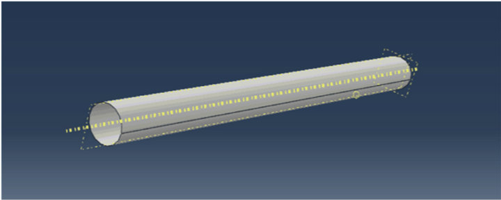
Figure 1. Abaqus Basic Pipe Model Simulation.
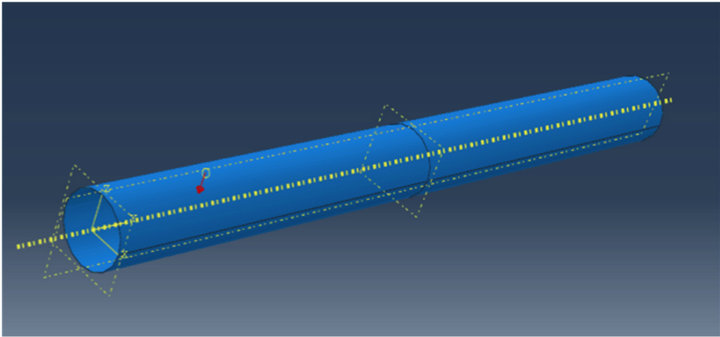
Figure 2. Abaqus Load Demonstration.
to reality by constraining the structural response to the applied load and a fixed constraint at a certain location. Therefore, there is a rigorous requirement that the correct boundary conditions be specified before conducting the analysis. The material properties used in the modeling are elastic and isotropic properties, in terms of stiffness and strength and the defect parameter, where  represents the distance the hole is from the end of the tube, and
  represents the diameter of the hole. The outputs of the model are acceleration, displacement, and velocity in the time domain. Collected data was analyzed and compared with experimental results.
4. Experimental Setup
An experiment to detect the hole in the carbon steel pipe was conducted in the laboratory. The experimental consists of carbon steel pipe, a hummer, charger amplifier, data acquisition and Accelerometer. The experimental setup, shown in Figure 5" target="_self"> Figure 5 included a carbon steel tube with a wall thickness of 0.35 cm, a diameter of 10 cm, and a length of 100 cm.
5. Analysis Techniques
Statistical methods included kurtosis, (ku), standard deviation (sd) are a time-domain analysis techniques and Fourier analysis method (FFT) is a frequency domain analysis technique. They are commonly used to analyze vibration signals or acoustic and to assess the severity of any damage.
5.1. Variance
The variance technique was used as shown in Figure 6. The equation of Variances is:

Figure 3. Basic Model Load Conditions.
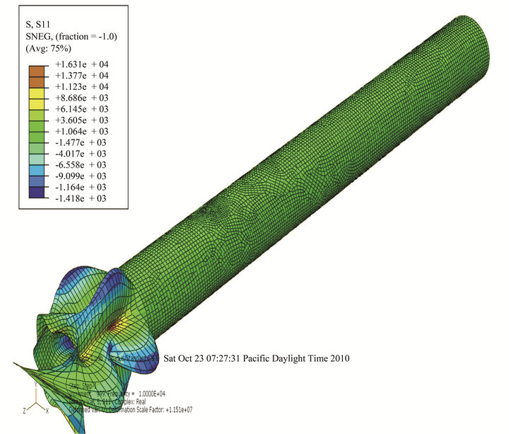
Figure 4. Load and Boundary Conditions Definitions of the Basic Model.
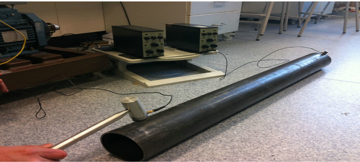
Figure 5. Carbon steel pipe specimen.
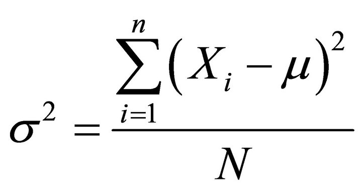 (4)
(4)
The value of variance remains constant for healthy and faulty (1 mm hole), after that, it increases up to (0.2254) and then decreases up to (0.0005) that is mean, variance parameter is not suitable to predict the fault.
5.2. Standard Deviation
The SD is the square root of the variance. It indicates the spread of the data, the larger the SD the more widely the data are spread out. Although influenced by extreme values, the SD is important in many tests of statistical significance:
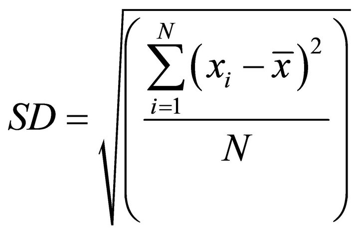 (5)
(5)
where xi a set of samples, N is the total number of samples, and ![]() is the mean value of the samples.
is the mean value of the samples.
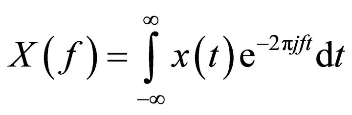
5.3. Fast Fourier Transform (FFT)
This is a technique for transforming the signal from timedomain to the frequency-domain. The mathematical formula is:
 (6)
(6)
where  is a continuous signal in time domain,
  is its Fourier transform and f is the frequency variable.
Simulation and experimental data collected and methods based on time and frequency techniques have applied for healthy and faulty cases of tested pipe for fault detecting.
6. Results and Discussions
The aim of this study is to detect and diagnose the faults in the pipe. The time-domain vibration signals collected from pipe as analyzed using variances and standard deviation as shown in Figures 6 and 7. As can be seen from figures there are fluctuations with the change of pipe condition between healthy and faulty signals. These fluctuations may lead to an incorrect decision for pipe condition and cannot be used to diagnose system defects. The time domain methods results of the experimental and simulation vibration signals have shown that such measures are not suitable for detecting faults in carbon steel pipe. Therefore, frequency domain (FFT) is employed to determine its effectiveness in detecting faults.
Frequency response measurements are a type of model testing which can be used to determine the resonant frequencies of a structure. Frequency response testing is accomplished by exciting a system with a known input and simultaneously measuring the corresponding output response.
Fast Fourier Transform (FFT) was applied for healthy and faulty collected data then plotted to determine the resonance amplitude. The “Healthy” pipe accelerometer results records of the vibration signatures in the frequency domain are shown in Figure 8" target="_self"> Figure 8. It shows the signature of a “healthy” pipe’s resonance frequency in the first mode of 500 Hz.
Experimental signal in healthy case was compared with simulation signal generated using ABAQUS software program. The result shows a good agreement between simulation and experimental signals using FFT method.
Fast Fourier Transform method was applied on simulation signals collected under different condition of the pipe (1 mm hole, 2 mm hole, 3 mm hole and 4 mm hole). The results are shown on Figures 9-13. Figure 9 demonstrates the modeling simulation of (a) time domain and
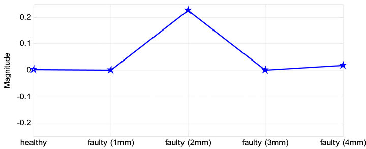
Figure 6. Statistical analysis-variance.
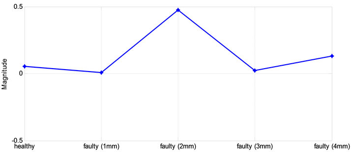
Figure 7. Statistical analysis-standard deviation.
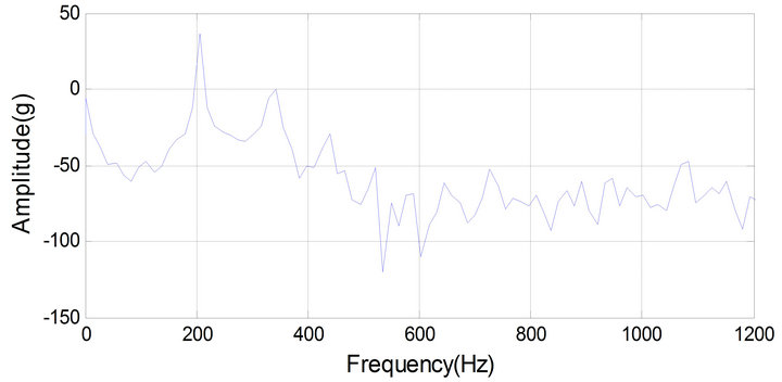
Figure 8. Experimental result-healthy.
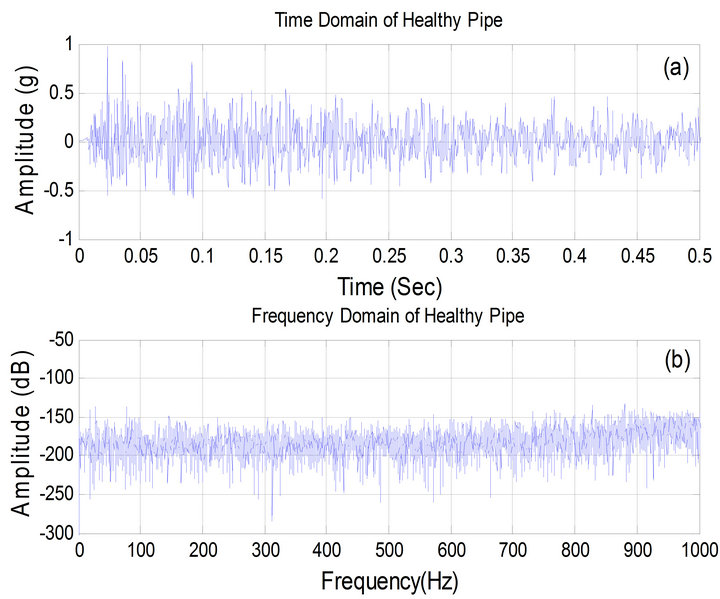
Figure 9. Vibration data for healthy pipe, (a) time domain, (b) frequency domain.
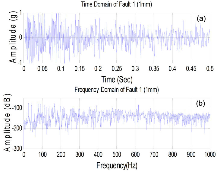
Figure 10. Vibration data for fault 1, (a) time domain, (b) frequency domain.
(b) frequency domain for the healthy pipe. At 500 Hz, which is “healthy” pipe’s first resonance frequency mode, notice that the amplitude is (−155 dB) that means it is 92% matching the experimental results (−143 dB). Therefore, it is feasible to build on that agreement to simulate more defects.
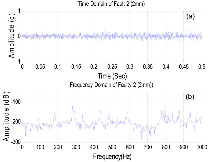
Figure 11. Vibration data for healthy pipe, (a) time domain, (b) frequency domain.
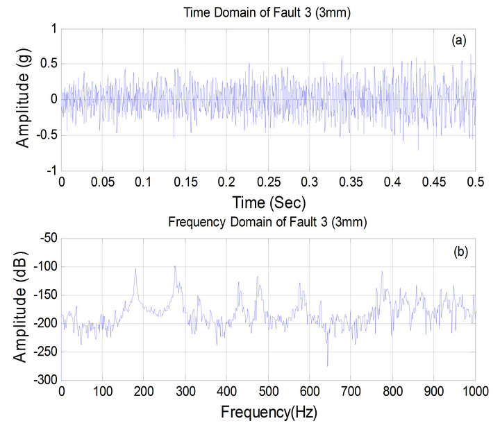
Figure 12. Vibration data for fault 3, (a) time domain, (b) frequency domain.
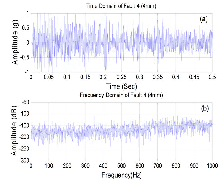
Figure 13. Vibration data for fault 4, (a) time domain, (b) frequency domain.
Figure 10 is vibration data for fault 1 mm, (a) Time domain, (b) Frequency domain. At 500 Hz, the frequency domain amplitude decrease (−25 dB) to become (−170 dB).
Figure 11 is vibration data for fault 2 mm, (a) Time domain, (b) Frequency domain At 500 Hz, the frequency domain amplitude decrease (−45 dB) to become (−200 dB).
Figure 12 is vibration data for fault 3 mm, (a) Time domain, (b) Frequency domain At 500 Hz, the frequency domain amplitude decrease (−65 dB) to become (−220 dB).
Figure 13 is vibration data for fault 4 mm, (a) Time domain, (b) Frequency domain At 500 Hz, the frequency domain amplitude decrease (−85 dB) to become (−240 dB).
Finally, the experimental and Abaqus modeling results were compared to examine the degree of agreement between the laboratory results and the theoretical results. Consequently, the results were assessed to determine whether it was reasonable and defensible to conclude that the size of the hole could be accurately predicted by conducting such a simple test of the pipe.
Based on results shown above there is a clear difference in the graphs based on pipe condition (healthy or damage) and graphs changes as per the nature of the tube defects situation. The greater the aperture size, the more significant the change in the shape of the graph is.
7. Conclusion
The main aim of this research was to study the natural response at different pipe conditions and to develop an inexpensive, reliable NDT method to diagnose faults related to carbon steel pipe. From the result it has been shown that the conventional techniques are not sufficient to reliably detect different types of faults in early stages and given detail information about their conditions as proven above by three different conventional techniques, whilst FFT is suitable method for analysing collected data. The proposed condition monitoring approach is based only on analyzing frequency response and does not require or depend on physical inspections. Also, it can be used to identify defective piping system supports, incurrectly placed supports, and the locations of maximum deflection requiring additional supports. The propose technique offers significant advantages such as avoidance of intrusive techniques and operator dependency and ability to measure the actual changes in the pipe hole and general applicability for any geometry or wall thickness. The experimental devices and modeling software used in this study achieved the main research objectives.
REFERENCES
- J. Hu, L. Zhang and W. Liang, “Detection of Small Leakage from Long Transportation Pipeline with Complex Noise,” Journal of Loss Prevention in the Process Industries, Vol. 24, pp. 449-457. doi:10.1016/j.jlp.2011.04.003
- D. N. Sinha, “Acoustic Sensor for Pipeline Monitoring,” Technical Report, Gas Technology Management Division Strategic Center for Natural Gas and Oil National Energy Technology Laboratory, Morgantown, 2005.
- Y. Khulief, A. Khalifa, R. Mansour and M. Habib, “Acoustic Detection of Leaks in Water Pipelines Using Measurements inside Pipe,” Journal of Pipeline Systems Engineering and Practice, Vol. 3, No. 2, 2012, pp. 47-54.
- F. Hao, A. Yang, J. Shijiu and Z. Zhoumo, “Desensitization Elimination in Pipeline Leakage Detection and Pre-Warning System Based on the Modeling Using Jones Matrix,” 2010 IEEE on Sensors Applications Symposium (SAS), Tianjin, 23-25 February 2010, pp. 101-104.
- Y. Jin, W. Yumei and L. Ping, “Information Processing for Leak Detection on Underground Water Supply Pipelines,” 2010 Third International Workshop on Advanced Computational Intelligence (IWACI), Chongqing, 25-27 August 2010, pp. 623-629.