Engineering
Vol.5 No.5A(2013), Article ID:31801,11 pages DOI:10.4236/eng.2013.55A003
On Point-Based Haptic Rendering
Experimental Robotics and Haptics Laboratory, Simon Fraser University, Burnaby, Canada
Email: payandeh@sfu.ca, wsa16@sfu.ca
Copyright © 2013 Shi Wen, Shahram Payandeh. This is an open access article distributed under the Creative Commons Attribution License, which permits unrestricted use, distribution, and reproduction in any medium, provided the original work is properly cited.
Received January 22, 2013; revised February 25, 2013; accepted March 3, 2013
Keywords: Haptic Rendering; Computational Mechanics; Point-Based Modeling; Level-of-Details
ABSTRACT
Haptic rendering is referred to as an approach for complementing graphical model of the virtual object with mechanicsbased properties. As a result, when the user interacts with the virtual object through a haptic device, the object can graphically deflect or deform following laws of mechanics. In addition, the user is able to feel the resulting interaction force when interacting with the virtual object. This paper presents a study of defining the levels-of-detail (LOD) in point-based computational mechanics for haptic rendering of objects. The approach uses the description of object as a set of sampled points. In comparison with the finite element method (FEM), point-based approach does not rely on any predefined mesh representation and depends on the point representation of the volume of the object. Different from solving the governing equations of motion representing the entire object based on pre-defined mesh representation which is used in FEM, in point-based modeling approach, the number of points involved in the computation of displacement/deformation can be adaptively defined during the solution cycle. This frame work can offer the implementation of the notion for levels-of-detail techniques for which can be used to tune the haptic rendering environment for increased realism and computational efficiency. This paper presents some initial experimental studies in implementing LOD in such environment.
1. Introduction
Interactive virtual training environment has been gaining a great popularity over the past decades. One of the main challenges of such development is the modeling of deformable objects such as soft tissues, organs, tendon, and skin. The two main requirements for modeling of such objects is the availability of material and biological properties and the need for the efficient/fast computational framework for achieving an interactive computational frame rate. In general, when interacting with the rigid model of the virtual object, the computational framework should support the graphic rendering rate of 20 - 30 Hz and the haptic force feedback rate of about 1 KHz [1]. However, when interacting with deformable or flexible objects, the force feedback rate can be comparably reduced in order to create a realistic haptic feedback. Developing an efficient and realistic computational model of deformable object is one of the main challenges for achieving an efficient haptic interaction environment.
Two main approaches have been followed in the past for modeling deformable objects. One of the approaches is based on the mass-spring methodology which represents the object as discretized mass points with spring connectivity. For example, [2,3] modeled a 1D suture object, and [4-7] modeled a deformable cloth-like object representing soft tissues. In general mass-spring modeling approach offers a simple and computationally efficient framework for developing interactive virtual training environment. Another approach for modeling deformable or flexible objects is based on finite element methods (FEM) and its various extensions. For example, [8] presented a simplified computational set-up for realtime simulation of soft tissue, [9-11] presented a fast linear solution for real-time user interaction with deformable objects. In general, due to the existence of large sizes of system matrices and the definition of shape functions, most of the solution approaches require an increased computational load which is in general not suitable for realtime interactive applications. For example, [12] developed an algorithm for enhancing the computational efficiency of the solution which still results in a very with limited extension to an interactive application.
Given the material properties of the object (e.g. Young’s module and Poisson ratio), FEM can still offer a more accurate representation of the physical objects in comparison with the mass-spring model. The main challenge of implementing FEM remains to be the design and development of a fast an efficient computational framework which may allows real-time application in the area of multi-modal haptic user interaction.
An approach for modeling deformable objects is referred to as the meshless method [13] which uses descretized element nodes (or points) to construct the object and uses the governing equations of motions through usage of radial basis weighting functions. [14] presented one of the earlier meshless methods in physics-based animation of objects. [15] presented a meshless elastic and plastic deformation framework. [16] proposed a meshless paradigm for modeling the point-sampled deformable object in real time. [17] proposed a similar meshless framework for modeling multiple deformable objects for user interaction purposes. One of the extensions of meshless method is referred to as the point-based (or particlebased) approach. [18] proposed a point-based modeling approach for graphic simulation of elastic and plastic objects. [19] presented a point-based approach for animating elasto-plastic solids, where a novel computational scheme based on displacement gradient is introduced using neighborhood optimization. In this analysis it was shown the point-based approach can give comparable results to that of approach based on FEM and hence can be used as an accurate representation and solution in haptic interaction [20]. In this paper, we demonstrate the implementation of a similar approach suitable for haptic rendering. Comparing with mass-spring model, the pointbased approach incorporate the material properties object implicitly in the modeling framework which has a significant advantage on the degree of accuracy of model. Comparing with FEM, the proposed modeling formwork can be potentially applied to real time rendering applications by adaptively including sample points in the computational model at the interactive rate.
The paper is organized as follow: Section 2 presents an overview of the point-based computational mechanics; Section 3 presents a definition for LOD which was used in this paper; Section 4 presents some experimental studies of our proposed LOD and Section 5 presents some concluding remarks.
2. Point-Based Mechanics
Point-based approach discretizes the control volume of the object into distributed points with no predefined connectivity or meshes (Figure 1). In contrast to FEM which defines an interpolation function (shape function) between the fixed defined nodes associated with a particular element [21], in point-based approach, functions such as Radial Basis Functions (RBF) is selected for interpolation of a continuous function based on a set of distinct arbitrary sample points defined in the control volume of the object [22].
Initially, through a weighting function, each point is defined to have a given mass in relation to its neighbor points. This given mass is computed by dividing the mass of the object by the number of points which needs
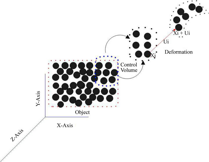
Figure 1. Illustration of the point-based mechanics model. The volume of the object is discretized into points. The actual deformation of the object is achieved by the deformation of each points inside the control volume.  is the position vector of the
  point,
  is its new position after being deformed by the displacement vector
 .
.
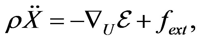
to be maintain during each solution cycle. The governing equation of motion of the object can be written as:
 (1)
(1)
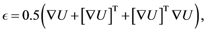
where  is defined as the spatial gradient of strain energy function with respect to displacement vector. The following equation defines the computation of strain which is used in the definition of
 ![]() (strain energy function).
(strain energy function).
 (2)
(2)
where  is the displacement vector of a point.
One of the main computational challenges for the solution of Equation (1) is the computation of the gradient ( ) defined in the Equation (2). In RBF approaches, Smoothed Particle Hydrodynamics (SPH) [23] is commonly used for the numerical computation of gradient function. Moving least square (MLS) is a computational tool belonging to the RBF methodologies which reconstructs continuous functions from a set of unorganized point samples (discrete points). In addition, a weighting function can be defined to weight the least squares measure and bias the computation towards the region around a point at which the reconstructed value is being evaluated [24,25].
The selection of weighting functions used in the computational model plays a very important role. In modeling deformable and flexible objects, there are several criterion which can be used for choosing a suitable weighting function. First the value of the weighting function should always be positive since for example, the mass and density of points are always defined as a positive integer; secondly, the weighting function should be decreasing in its value when the distance between the reference point and its neighbor points increases (i.e. the influence is local and vanishes as the distance increases).
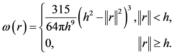
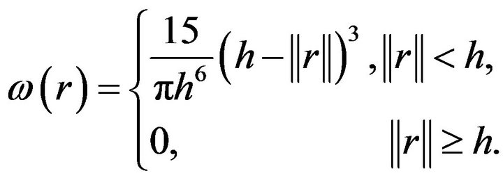
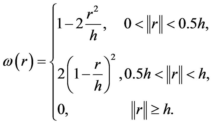
In general, several weighting functions can be defined which is a modified version of composite quadratic tensor-product weight function defined in [26,27]. Some examples can be:
 (3)
(3)
 (4)
(4)
 (5)
(5)
 (6)
(6)
where  is the distance between any two points (i.e. one being a reference point) and
  is a defined cut-off value. The cut off value
  in the weighting function has two main purposes. First, when
  is decreasing, it localizes the weights to points which are within the reduced neighborhood of the current reference point. When
  increases, it can offer a uniform and smooth contribution to the neighbor points. In general, weighting functions (4) and (5) are used for fluid modeling. (4) is used for solving a class of particle clustering problem and (5) is used for viscosity computation. (6) is also for modeling elastic object.
As an example, in Equation (1), the density of each point i is computed as:
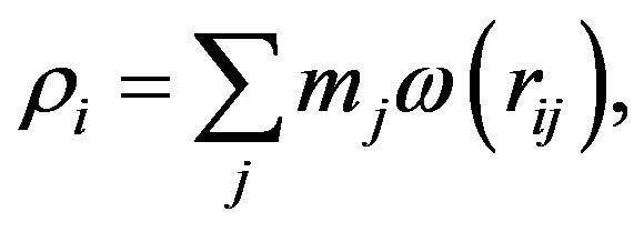 (7)
(7)
where ![]() is the distance between point
is the distance between point  and
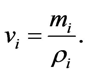
and . The volume of each point can now be computed as:
 (8)
(8)
In Equation (2), the gradient of the displacement is defined as:
 (9)
(9)
where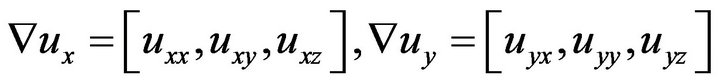 , and
, and
 are the three row vectors denote the derivatives with respect to (x, y and z).
Using MLS, the basic idea is to expand the displacement about a point  using Taylor Series expansion and define the displacement of the adjacent points in terms of the current point and up to the first order expansion of the series. The interpolated displacement is then define by value which minimizes the square of the error (Appendix). The overall computation results of
  evaluated at the
  point can be written as:
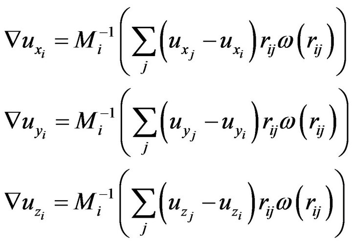 (10)
(10)
where for example, 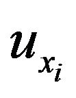 denotes the x-component of the displacement vector at the
  point.
In the above  is a 3 × 3 matrix which can be precomputed at point
  and defined as:
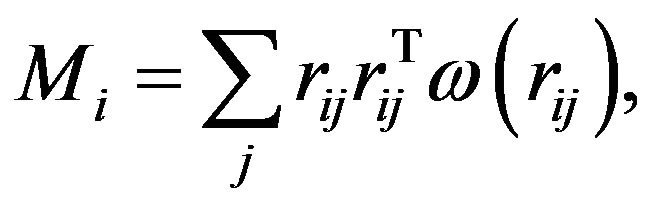 (11)
(11)
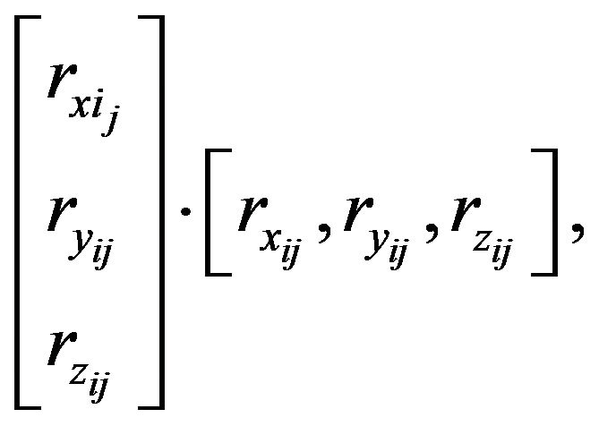
where ![]() is a distance vector between points
is a distance vector between points  and
and  expressed in the reference coordinate frame. Given the value strain from Equation (2) the strain energy stored computed at a point
  can be written as
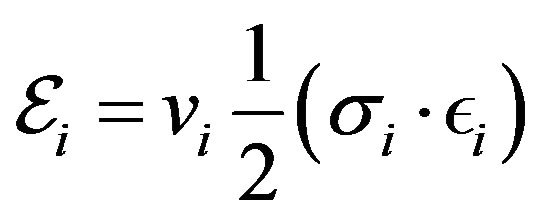 .
.
The body force  defined by
  used in Equation (1) is a function of displacement vector at point
  and the displacements of all the neighbors
 . Taking the derivative with respect to these displacements yields the forces acting at a point
  and all its neighbors
 :
:
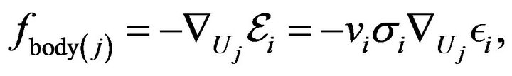 (12)
(12)
where  is the body force at a point
 ,
,  is the strain energy at a point
  and
and ![]() is the volume of a point
is the volume of a point . Based on Newton’s third law, the body force acting on a point
  is computed as the negative sum of all the body forces acting at its neighbor points,
 (13)
(13)
Using the expression for  and
and , we can determine the final expression of
 . The final expressions for the internal body forces can be written as:
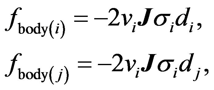 (14)
(14)
where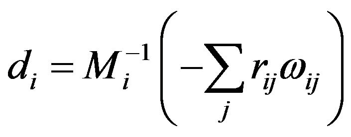 , and
, and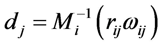 ,
, ![]()
and  are the volumes of the points
  and
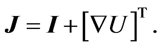
and . In the above expression, the Jacobian matrix
 ![]() is computed from:
is computed from:
Preliminarily Comparison Study
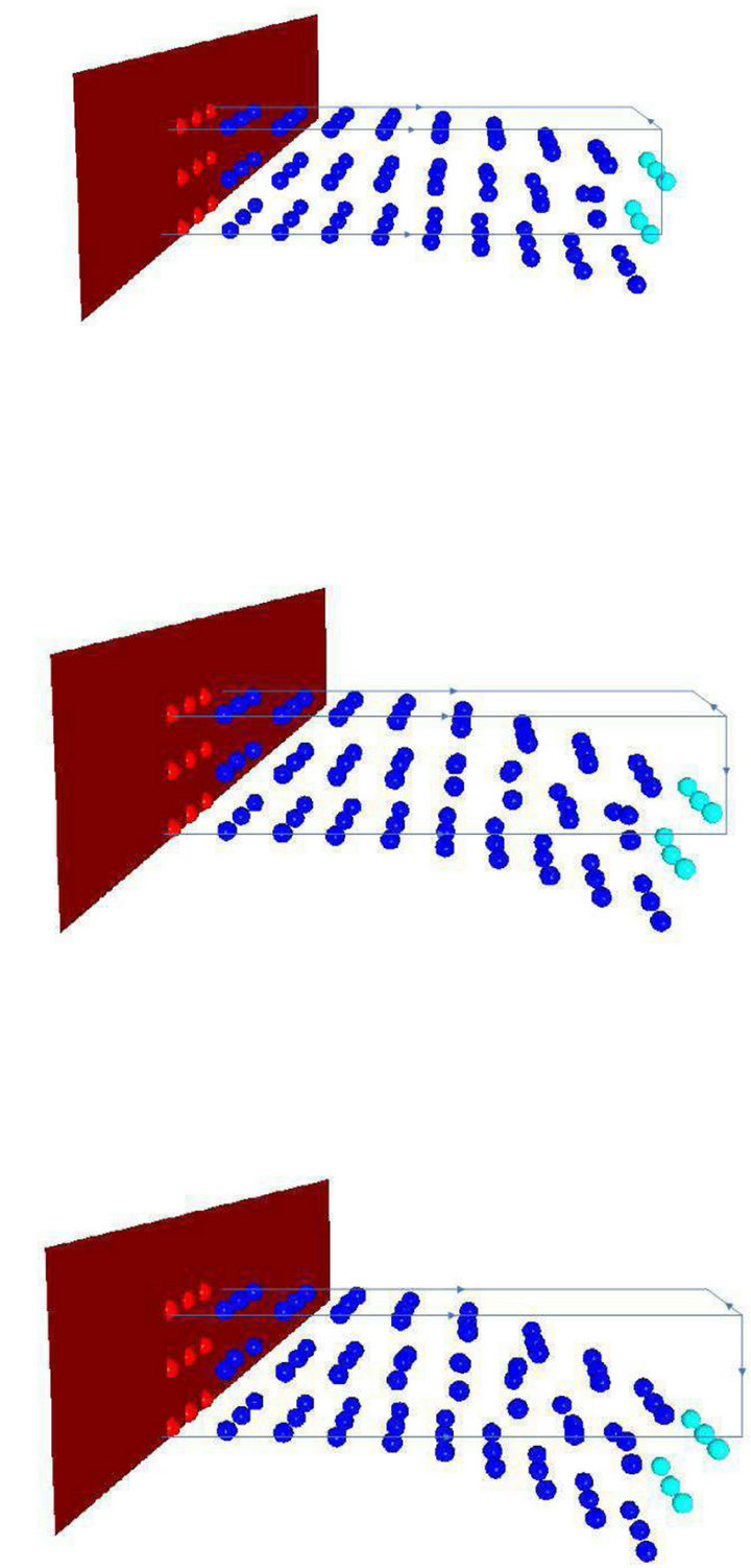
In this section, we present the results of a haptic interaction environment based on the proposed framework. We also present some comparison study of evaluating tip deflection of the cantilever bean under constant load using point-based mechanics and FEM. The experimental setup consists of a desktop computational platform with Intel P4 3.0 GHz CPU, 1G RAM and the Phantom Omni haptic device. We define a collection of rectangular cross sectional objects composed by 90 points ((3 × 3 × 3)) points per cross section). The foundation points are evenly distributed with the spatial distance between each point of 0.015 m. In this experiment, both ends of the objects were fixed and represented with the red spheres.
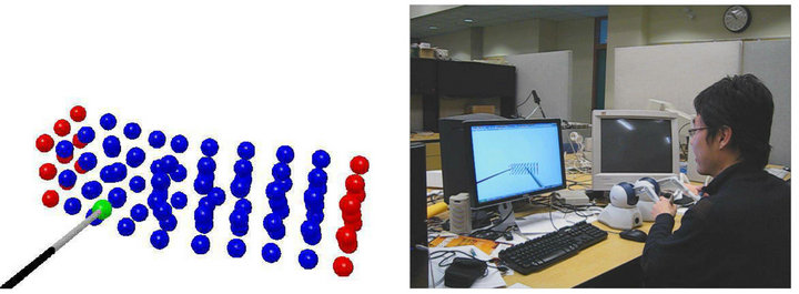
In our experiment, we study the effect of different weighting functions defined in Equations (3)-(6). For example, Figure 2(a) shows the computation of foundation points based in the weighting function defined in Equation (3). This Figure also shows a virtual probe which represents the presence of the user in the haptic rendering environment. As shown in Figure 2(b), the user can interact with the point-based model of the block through haptic feedback device. When the contact is made between the virtual probe and the object, the point-based model of the object can deform and the resultant interaction forces is feb-back to the haptic device. In this Figure, green sphere represent the contacted point which the user is interacting with. Figure 2(c) shows and example of such haptic interaction. The Figure shows a plot of haptic force which was fed-back to the user over the duration of a part of the experiment.
In order to validate the computational model of the object based on the point-based mechanics approach, we conducted an experimental comparison with a commercially available standard FEM package. Our experimental model is similar to our haptic interaction model except we have constrained one end of the block while making the other end free of any constraints (i.e. a cantilever model). We have selected Young’s Modulus to  Pa and Poisson’s ratio to 0.4. For the point-based mechanics model, we also have selected the cut off distance,
  , in Equation (3) to be 0.1 m. At each experiment, we have recorded the shape and the tip deflection of the model under a constant load. For the FEM, we also have defined the same object using the same boundary conditions and loading condition using a commercial FE software Comsol (http://www.comsol.com/). Figure 3 shows both the visualization and the results of our comparative study.
Figure 4 compares the magnitude of the deflection of a point at the tip of the cantilever. The axes are the magnitude of deflection under four constant load conditions. As it can be seen, under the same constant tip load force, both methods can yield to comparable results.
3. Definition of Levels-of-Detail
The proposed framework offers an approach where global deformation of an object can be computed using small number of points used in the local deformation solution. In order to establish relationships between the global and local deformation of object as a function of the sampled points, we study how the resolution of the object base model (i.e. object defined by foundation points) can affect the haptic frame rate through increasing the reso-
 (a)
(a)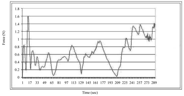 (b)
(b)
Figure 2. Experimental results of haptic interaction with a deformable model. In the experiment, the users presence in the virtual scene is represented by a cylindrical probe. Points in red are boundary points; Points in green is the point being dragged by the probe; Points in blue are points which deform due to the action of the probe. (a) The experimental result of weighting function defined in 3; (b) Shows a user manipulate the point-based object through haptic device; (c) Haptic force feedback profile fed-back to the user through the haptic device.
lution of the base point. The major computational challenge in our approach is the computation of the displacement gradient tensor  for each of the points. Intuitively the basic approach is that we assume that the local deformation affects the points closer to the contact region. The contact force propagate through-out the body and the resultant internal forces are less propagated to the points beyond certain threshold. A localization or levels-of-detail (LOD) can be then be implemented to capture the above motivation where one should be able to both increase the realism of the haptic interaction while maintaining a high haptic rate. We propose an approach by defining influence ranges as a function of the distance of a point from the contact area. For example, in Figure 5 and at the instant of contact a dense sample of points of object inside a volume located at the tip of a probe can be considered as points located at the proximity of the contact area.
The local and internal deformation can propagate from the contact region to points defining the boundary of the object. Our initial algorithm associates the larger radius of propagation influence to smaller number of points being sampled from the foundation points comparing to the in between regions. We proposed a pseudo-random point selection algorithm which selects points within preset ranges/radii under pre-defined weighting factors defined through a random number generator. For example, the selection weighting factor for the localization range (i.e. range within the contact area) is set to be large since we require a high density of points in this range. On the other hand, the selection weighting factor for the influence range is set to be small since we only need a limited number of points to propagate the deformation from the contact region to the boundary points. This approach is analogous to the LOD scheme used in the finite element model, where the mesh density varies from fine mesh in
 (a)
(a)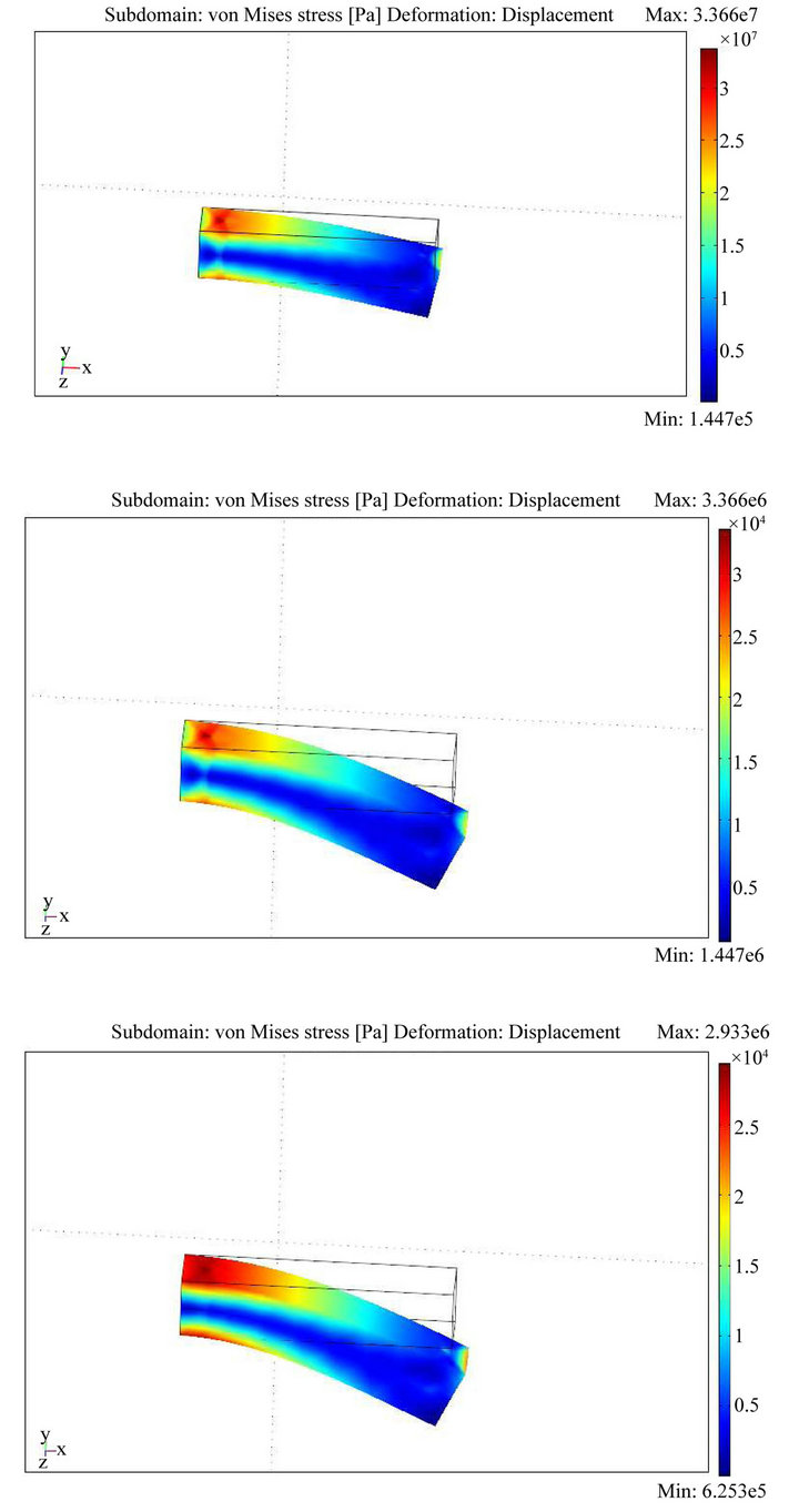 (b)
(b)
Figure 3. Comparison between point and FEM based elastic cantilever deflection. The display in the left column shows deflection results based on point based model; results in the right column illustrate the deflection results based on FEM. Both results are obtained using constant Young’s Modulus and Poisson’s ratio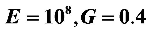 . The first row shows the deflection under constant load vector F = (0,1000,0), the second row is for of along with the constant load force vectors are as follows: for the first case in row one Y = 108, G = 0.4, F = (0,1000,0); The second case in for F = (0,10000,0) and the third row is for load vector F = (0,10000,0).
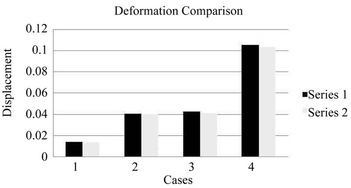
Figure 4. Comparison of the magnitude of deflection between the point-based and FEM models. The deflection data was collected on the upper right point in the front face of the end tip. The black bars represent displacement under the point-based model, white bars indicate displacement based on FEM.
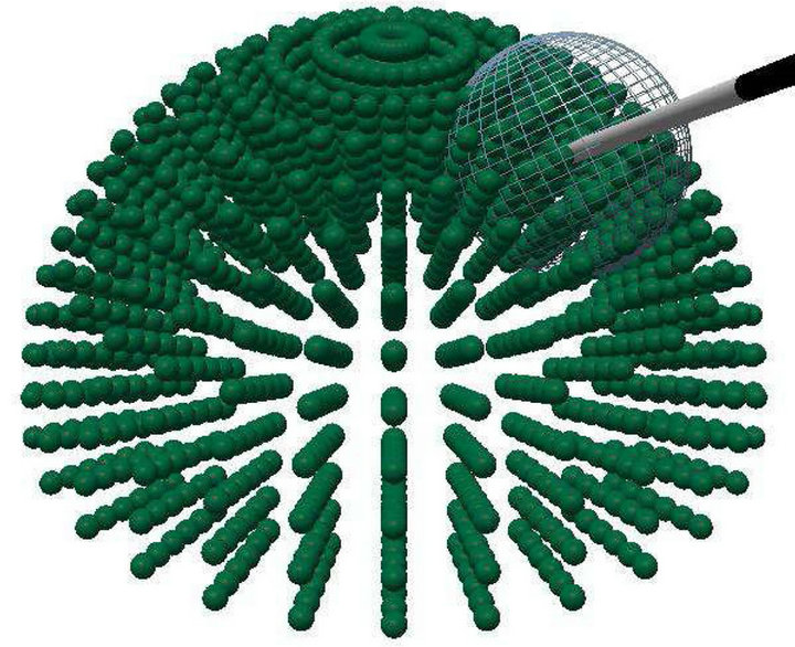
Figure 5. Level-of-detail schematic, contact between the tip of the probe and the points within the half sphere object is detected by a sphere-sphere collision detection algorithm. Neighbor points that fall within the influence range will be selected and incorporated into the computational model for deformation rendering.
the region of interest to the coarse mesh in the boundary region. Figure 6 illustrates the schematic of the localization distance threshold. The points are selected based on their distance to the point of contact.
We define localization distance  to be a linear function of the cut-off distance
 , and we use two different constants (
 and
and ) to define the threshold of the localization distances
  as the selection ranges. Once being defined,
  and
and  will remain constant through-out the computation. Similarly, we define propagation distance,
  , where
  indicates the
  level of propagation. We also define
  to be a linear function of
 . By changing the constants
 , the threshold distance of each propagation level can vary.
Once the contact is detected, the dynamic selection algorithm initiated to select the points in terms of the contact region and the propagation of deformation. After the selection, we incorporate selected points into the computation model and render the deformation effect. The selection function first generates a random number  between 0 and 10 and determines the selection weighting factor. Then, it determines the distances between the current positions of neighbor points and the contact point. After that, it selects the points by comparing the distances with the threshold distance based on the selection weighting factor. If the distance is less than
 , the selection weighting factor is 1, and the point is directly selected. If the distance is between
  and
and , the weighting factor of selection is 0.8 (the probability of
  is
is ). The points within the propagation levels are also selected based on the weighting factor of the propagation level
 .
.  is a monotonically increasing integer in terms of propagation level
 , which controls the weighting factor of the propagation points being selected. The weighting factor of selection for level
 is
is . The upper bound of
  is set to be 10.
Experimental Analysis
We conduct an experimental study to compare and analyze how the number of the propagation levels and the selection factors can affect the LOD model in haptic rendering. Figure 7 shows the initial foundation points which were used to represent the experimental object. Figures 8 and 9 show some examples of our experimental results comparing the different propagation levels and their selection weighting factors along with the system update rate. In the experiment, we apply a constant pulling force at the 111th point in the model, and plot the magnitudes of the displacements of all the points in the model at the 9th second in run time. The localization distances  and
and  remain unchanged and the selected

Figure 6. Schematic of the point-based LOD model. A virtual probe is contacting an object, and the blue point is the contact point. Two localization distances  and two propagation distances
  are initialized.
  is the last propagation distance which can include all the boundary points. Red points are the boundary points; Points selected by the algorithm are shaded in black.
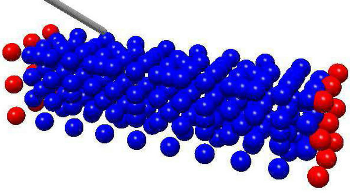
Figure 7. Foundation points representing the object used in the proposed LOD studies.
neighbor points are shaded in brown and blue.
We analyze how different cut-off distances  of the localization can affect the frame rate in the LOD model. Table 1 compares the run time of the different localization cut off distances on different foundation points. As we increase the distance thresholds
  and
and , the rendering time per frame increases since more points are incorporated into the computation of deformation.
4. Conclusion
One of the main challenges of haptic rendering of virtual objects is methods for their realistic representation which can also offer a fast interactive computational framework. This paper investigated an approach which can be a bridge
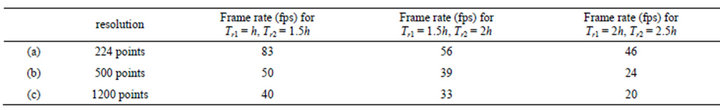
Table 1. Analysis of the proposed point-based LOD in haptic rendering.
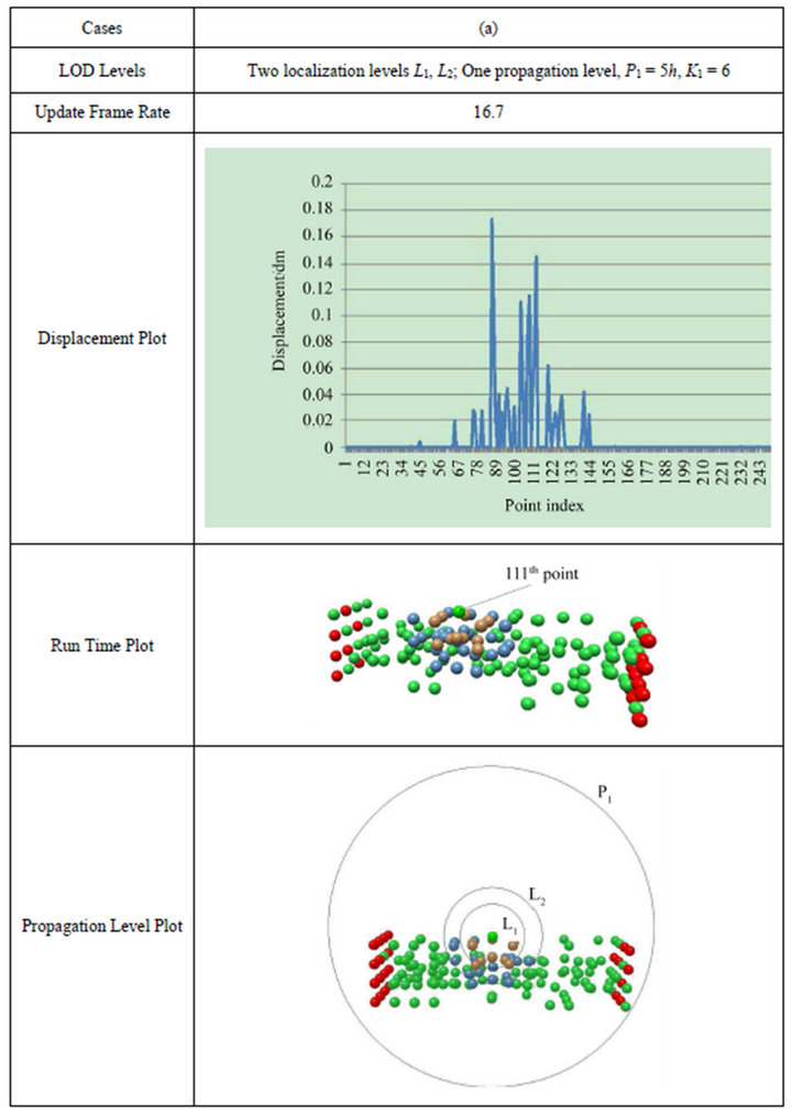
Figure 8. Comparison of different propagation level setups. First row is the definition of the propagation level; Second is the associated frame rate; Third row is the displacement plot of the points; Fourth row is the visualization of the displacement; Fifth row is the schematics of the propagation level. In this experiment, we have defined one propagation level with low selection weighting factor (0.4). The local points are colored in brown and dark blue, the propagation points are colored in green.

Figure 9. Comparison of different propagation level setups. First row is the definition of the propagation level; Second is the associated frame rate; Third row is the displacement plot of the points; Fourth row is the visualization of the displacement; Fifth row is the schematics of the propagation level. In this experiment, we have defined one propagation level with low selection weighting factor (0.2). Brown and dark blue points are local points and green points are propagation points.
between the realism and computational efficiency. The paper presents an overview of point-based mechanics approach and also demonstrated its implementation in a typical haptic interaction environment. In addition it is shown that the point-based mechanics approach can be defined and modeled which can give a comparable computational results to that of standard FEM. Another key advantages of the point-based method is that one can initialize a control volume of an object with collection of points where only subset of these points can be sampled during the simulation process. This is an important feature since during the run-time of simulation process, one can adaptively sample more points in the computational model for increased accuracy. In this paper, we investigated a 3D point-based object modeling approach for haptic rendering. It was shown that this approach can offer a comparable results to that of the FEM [20]. The proposed framework allows interaction where user can manipulate the point-based object model using a haptic device. We present a notion of levels-of-detail (LOD) where foundation points which can represent the object can be grouped into different levels. For this early study, we have presented an approach were base on the distance of points from the contact area. Points can be populated with different densities in various geometrical regions away from the contact point while including regions defined by the boundary points. Feasibility of the proposed LOD approach was studied to investigate the practicality of the proposed approach in changing the resolution of the points during the haptic interaction. This framework allows both inclusion of the material properties of the object and also direct mapping to various medical imaging modalities where scanned point-clouds can be mapped to the haptic interaction framework.
REFERENCES
- K. Salisbury, F. Conti and F. Barbagli, “Haptic Rendering: Introductory Concepts,” IEEE Computer Society, 2004.
- M. LeDuc, S. Payandeh and J. Dill, “Toward modeling of a suture task, Graphics Interface(GI),” Halifax, Nova Scotia, 2003, pp. 273-279.
- H. F. Shi and S. Payandeh, “Real-Time Knotting and Unknotting,” IEEE International Conference on Robotic Automation (ICRA), Roma, 10-14 April 2007, pp. 2570- 2575.
- S. Payandeh, H. Zhang and J. Cha, “Toward Interactive Haptic Simulation of Cutting,” International Journal of Virtual Technology and Multimedia, Vol. 1, No. 2, 2010, pp. 172-186.
- H. Zhang, S. Payandeh and J. Dill, “On Cutting and Dissection of Virtual Deformable Objects,” Proceedings of IEEE International Conference on Robotics and Automation, New Orleans, 26 April-1 May 2004, pp. 3908-3913.
- W. Mollemans, F. Schutyser, J. V. Cleynenbreugel and P. Suetens, “Tetrahedral Mass Spring Model for Fast Soft Tissue Deformation,” IS4TM 2003, LNCS 2673, 2003, pp. 145-154.
- H. F. Shi and S. Payandeh, “On Suturing Simulation with Haptic Feedback,” Proceedings of 6th International Conference of Haptics: Perception, Devices and Scenarios, EuroHaptics, 2008, pp. 599-608.
- J. Berkley, S. Weghorst, H. Gladstone, G. Raugi, D. Berg and M. Ganter, “Banded Matrix Approach to Finite Element Modelling for Soft Tissue Simulation, Virtual Reality,” Springer, Berlin, 1999.
- J. Berkley, G. Turkiyyah, D. Berg, M. Ganter and S. Weghorst, “Real-Time Finite Element Modeling for Surgery Simulation: An Application to Virtual Suturing,” IEEE Transactions on Visualization and Computer, 2004, pp. 314-325.
- W. Maurel, “3D Modeling of the Human Upper Limb Including the Biomechanics of Joints, Muscles and Soft Tissues,” Ph.D. Thesis, Laboratoire d’Infographie—Ecole Polytechnique Federale de Lausanne, 1999.
- S. Marlatt and S. Payandeh, “Modelling the Effect of Rayleigh Damping on the Stability of Real-Time Finite Element Analysis,” Proceedings of World Haptics, Pisa, 18-20 March 2005.
- I. Peterlik and L. Matyska, “An Algorithm of State-Space Precomputation Allowing Non-Linear Haptic Deformation Modelling Using Finite Element Method,” Second Joint EuroHaptics Conference and Symposium on Haptic Interfaces for Virtual Environment and Teleoperator Systems, 2007.
- T. Belytschko, Y. Krongauz, D. Organ, M. Fleming and P. Krysl, “Meshless Methods: An Overview and Recent Developments,” Computer Methods in Applied Mechanics and Engineering, Vol. 139, No. 1-4, 1996, pp. 3-47.
- T. Fries and H. Matthies, “Classification and Overview of Meshfree Methods,” Technical Report, TU Brunswick, Germany Nr. 2003-03, 2003.
- M. Pauly, R. Keiser, B. Adams, P. Dutr, M. Gross and L. J. Guibas, “Meshless Animation of Fracturing Solids,” International Conference on Computer Graphics and Interactive Techniques, 2005, pp. 957-964.
- X. Guo and H. Qin, “Real-Time Meshless Deformation: Collision Detection and Deformable Objects,” Computer Animated Virtual Worlds, Vol. 16, No. 3-4, 2005, pp. 189-200.
- B. Adams, M. Wicke, M. Ovsjanikov, M. Wand, H.-P. Seidel and L. J. Guibas, “Meshless Shape and Motion Design for Multiple Deformable Objects,” Computer Graphics Forum, Vol. 29, No. 1, 2010, pp. 43-59. doi:10.1111/j.1467-8659.2009.01536.x
- M. Miller, R. Keiser, A. Nealen, M. Pauly, M. Gross and M. Alexa, “Point Based Animation of Elastic, Plastic and Melting Objects,” Eurographics/ACM SIGGRAPH Symposium on Computer Animation, 2004.
- D. Gerszewski, H. Bhattacharya and A. W. Bargteil, “A Point-Based Method for Animating Elastoplastic Solids,” Eurographics/ACM SIGGRAPH Symposium on Computer Animation, 2009.
- W. Shi and S. Payandeh “Towards Point-Based Haptic Interactions With Deformable Objects,” ASME World Conference on Innovative Virtual Reality, Ames, 12-14 May 2010, pp. 259-265.
- S. Payandeh and N. Azouz, “Finite Elements, MassSpring-Damper Systems and Haptic Rendering,” Proceedings of IEEE International Symposium on Computational Intelligence in Robotics and Automation, 29 July-1 August 2001, pp. 224-230.
- R. L. Hardy, “Multiquadric Equations of Topography and Other Irregular Surfaces,” Journal of Geophysical Research, Vol. 76, No. 8, 1971, pp. 1905-1915.
- J. J. Monaghan, “Smoothed Particle Hydrodynamics,” Annual Review of Astronomy and Astrophysics, Vol. 30, 1992, pp. 543-574. doi:10.1146/annurev.aa.30.090192.002551
- A. Nealen, “An As-Short-As-Possible Introduction to the Least Squares, Weighted Least Squares and Moving Least Squares Methods for Scattered Data Approximation and Interpolation,” Internal Report, TU Darmstadt, 1990.
- D. Levin, “The Approximation Power of Moving LeastSqaures,” Mathematics of Computation, Vol. 67, No. 224, 1998, pp. 1517-1531. doi:10.1090/S0025-5718-98-00974-0
- M. Miller, D. Charypar and M. Gross, “Particle-Based Fluid Simulation for Interactive Applications,” Eurographics/SIGGRAPH Symposium on Computer Animation, San Diego, 26-27 July 2003.
- X. Guo and H. Qin, “Meshless Methods for PhysicsBased Modeling and Simulation of Deformable Models,” Science in China Series F: Information Sciences, Vol. 52, No. 3, 2009, pp. 401-417. doi:10.1007/s11432-009-0069-x
Appendix
For derivation of the numerical solution of  used in Equation (1), we utilized use the simplified expression defined in Equation (10) which treats the 3 × 3 matrix as three row vectors,
  and
and  respectively. In the following, we define an approach where we can solve for these three vectors separately.
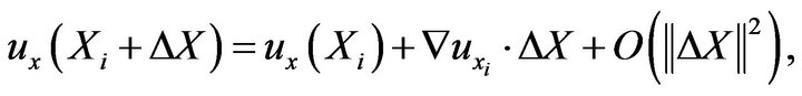
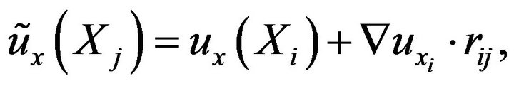
For example, let us evaluate the differential form of the x-component of the displacement vector . By definition, method based on MLS is first order accurate. Using the first order Taylor expansion of
  in the neighborhood of the
  point, we have:
 (15)
(15)
where  is the position vector of the
  point,
  is the small change in position,
  is the derivative
  evaluated at point
  which is written as
 .
.
Suppose that  and
and  are known. By replacing
  in Equation (15) using the distance vector
  between point
  and
and ,
,  of the neighbor point
  of point
  can be approximated as,
 (16)
(16)
where 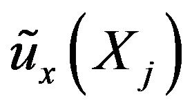 is the approximated value of
 . The measure of the error of the above approximation is given by a sum of the squared differences
(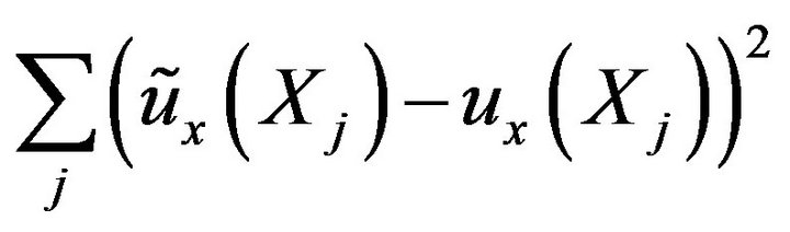 , since all the neighbor points j of point
  need to be taken into consideration and weighted by the weighting function
 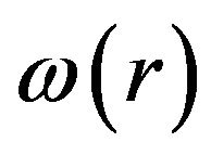 as:
as:
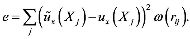 (17)
(17)
Substitute Equation (16) into Equation (17), we have:
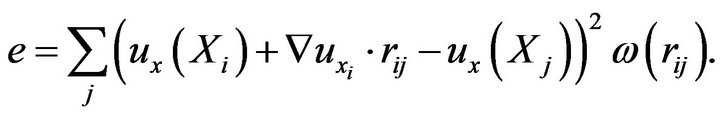 (18)
(18)
Given point  and its x-component displacement
 , the solution for the gradient
  is the one which minimizes the error
![]() . This becomes an optimization problem. By setting the derivative of
. This becomes an optimization problem. By setting the derivative of ![]() with respect to
with respect to  to zero we can write:
 (19)
(19)
We can solve for  as:
as:
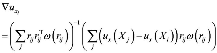 (20)
(20)
where 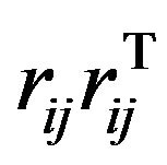 is computed as
 (21)
(21)
which is a 3 × 3 matrix. e.g.  is the x-component of distance vector
![]() ). The spatial gradient of the other two components of the displacement vector (
). The spatial gradient of the other two components of the displacement vector ( and
and ) can be computed in the same derivation. In the main context of the thesis, we use
  denoting
  and
and  denoting
  for simplicity.