Engineering
Vol. 4 No. 12 (2012) , Article ID: 25741 , 4 pages DOI:10.4236/eng.2012.412108
Kinematical Analysis and Simulation of High-Speed Plate Carrying Manipulator Based on Matlab
School of Mechanical Engineering, University of Yangzhou, Yangzhou, China
Email: wk15937945561@163.com, jpzhou@yzu.edu.cn
Received October 13, 2012; revised November 14, 2012; accepted November 23, 2012
Keywords: High-Speed Plate Carrying Manipulator; D-H Method; Robotics Toolbox; Trajectory Planning
ABSTRACT
In order to construct the more effective kinematics method for industry, by taking a high-speed plate handing robot as an example, the structure and parameters of the robot linkages are analyzed, and the standard Denavit-Hartenberg method is applied to establish the coordinates and the kinematic equation of the linkages. Depending on the graphics and matrix calculation ability of Matlab especially including the Robotics Toolbox, the handling robot has been modeled and its kinematics, inverse kinematics and the trajectory planning have been simulated. Therefore, the correctness of kinematic equation has been verified, meanwhile, the functions of displacement, velocity, acceleration and trajectory of all the joints are also obtained. In a further step, this has verified the validity of all the structure parameters and provided a reliable basis for the theoretical research on the design, dynamics analysis and trajectory planning of the manipulator control system.
1. Introduction
As a typical representative and a main technical means of information technology and advanced manufacturing technology, the complete set of automatic stamping processing line has become a high technology to which the developed countries have paid much attention. And its development level has become one of the most important standards to measure a nation’s technical development. It has been extensively applied in the industry of mechaniccal manufacturing, nuclear, aerospace, energy and transportation, petroleum chemistry, building, electronic and etc. [1]. But, one key aspect of the automatic stamping processing line is to develop a mechanical manipulator with the characteristic of the high-speed and dynamic transmission.
At present, the sheet metal forming production line is operated at the high productive rate of 15 - 25 SPM. Removing the time spent by the press stamping operations, there is only about 2 s left to the robot manipulator. In such a short period of time, the manipulator has to operate at a high speed of 200 - 250 m/min, so that the operations such as loading, moving and unloading can be fulfilled. And this has put forward higher requirements to the mechanical structure, material friction characteristics, and structural dynamic characteristics of the robot manipulator.
Taking a high-speed plate carrying manipulator as the research object, this paper firstly analyzes the structure and connecting rod parameters; then adopts the standard D-H method [2] to establish the kinematics equation; and then discusses the positive and inverse kinematics algorithm, and the trajectory planning problems; finally in the environment of Matlab, the kinematics model is built to take kinematics simulation by using of Robotics Toolbox [3]. In simulation process, we can not only directly observe the robot motion, but also get the required data in the graphic form. Therefore, the virtual performace of the product can be tested in the conceptual design stage, so as to improve the design performance, reduce design cost and decrease product development time.
2. The Structure Design and Link Parameters of High-Speed Plate Carrying Manipulator
2.1. The Design Requirements of High-Speed Plate Carrying Manipulator
2.1.1. The Workplace of High-Speed Plate Carrying Manipulator
The traditional stamping processing method relies on a stand-alone manual which is inefficient, inaccurate and insecurity. So it has already become increasingly unsuited to the requirements of modern mass production, especially when the requirements of the sheet metal processing annual output exceeds thousands tons, this contradiction is more prominent. The current stamping equipment is toward the trend of automation, sets and online development. With the rapid development of China’s market economy, especially in the coastal areas where the shortage of skilled workers is severe, and labor costs rises sharply, many machinery manufacturers have the urgent demand for manufacturing automation, and require machine and equipment manufacturing industry to provide users with a complete set of on-line technical services to improve production efficiency and reduce labor costs. Therefore, the development of the technology of sheet metal production line is even more important. One of the core technologies of sheet metal stamping equipment line is the design of high-speed plate carrying manipulator. As shown in Figure 1, it is high-speed plate carrying manipulator in the application of stamping processing complete sets of equipment on-line system.
2.1.2. The Operation Process of High-Speed Plate Carrying Manipulator
According to the composition of the stamping process sets of on-line system and the role of the high-speed plate carrying manipulator, the working cycle of a manipulator contains nine action process, as shown in Figure 2:
1) From the point of origin, the left electromagnetic valve is energized after pressing the start button, then the manipulator moves to the left. It won’t stop until it encounters the left limit switch.
2) Simultaneously the manipulator begins to drop after the decreased electromagnetic valve opens, then, it won’t stop until it encounters the lower limit switch.
3) At the same time the clamp electromagnetic valve is energized, then the manipulator is clamped.
4) After the rise electromagnetic valve is energized, the manipulator begins to rise, then it won’t stop until it encounters the rise limit switch.
5) Simultaneously the manipulator moves to the right after the right electromagnetic valve is energized, then, it won’t stop until it encounters the right limit switch.
6) Simultaneously the manipulator begins to drop after the decreased electromagnetic valve is energized, then, it won’t stop until it encounters the lower limit switch.
7) At the same time the clamp electromagnetic valve is opened, then, the manipulator is opened.
8) After the rise electromagnetic valve is energized, the manipulator begins to rise, then, it won’t stop until it
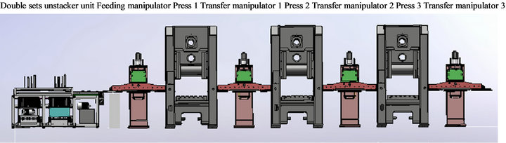
Figure 1. The composition of the stamping processing sets of on-line system.
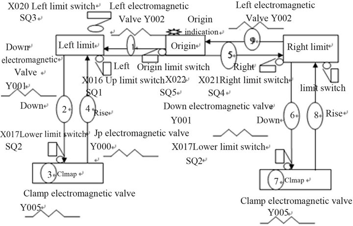
Figure 2. The operation process of the manipulator.
encounters the rise limit switch.
9) Simultaneously the manipulator moves to the origin after the left electromagnetic valve is energized, then, it won’t stop until it encounters the left limit switch.
So far, the manipulator after 9 step action completes a cycle of its movement, and then, it continues the cycle work.
Based on the above analysis, we have developed a three-dimensional model of the manipulator as shown in Figure 3, which can be used to analyze the dynamic characteristics of the manipulator.
2.2. The Design Parameters of High-Speed Plate Carrying Manipulator
2.2.1. D-H Transformation
In order to describe the translational and rotational relationships between adjacent rods, Denavit and Hartenberg (1955) have proposed a matrix method to establish the possessed coordinate system for each rod in the linkage chain. This method is to establish a homogeneous transformation matrix for each of the join bar coordinate, which represents the relationship of the previous coordinate system of the bar, and the principle [4,5] is detailed as follows:
OXYZ: A fixed reference coordinate system of the fixed coordinates, is called the coordinate system.
OiXiYiZi: Fixed connected with the member bar of number I of the robot, the origin of coordinate is at the center point of the joint of the I + 1th.
Identify and establish each coordinate system by following three rules.
1): Zi−1 axis along the motion shaft of the join of the i th.
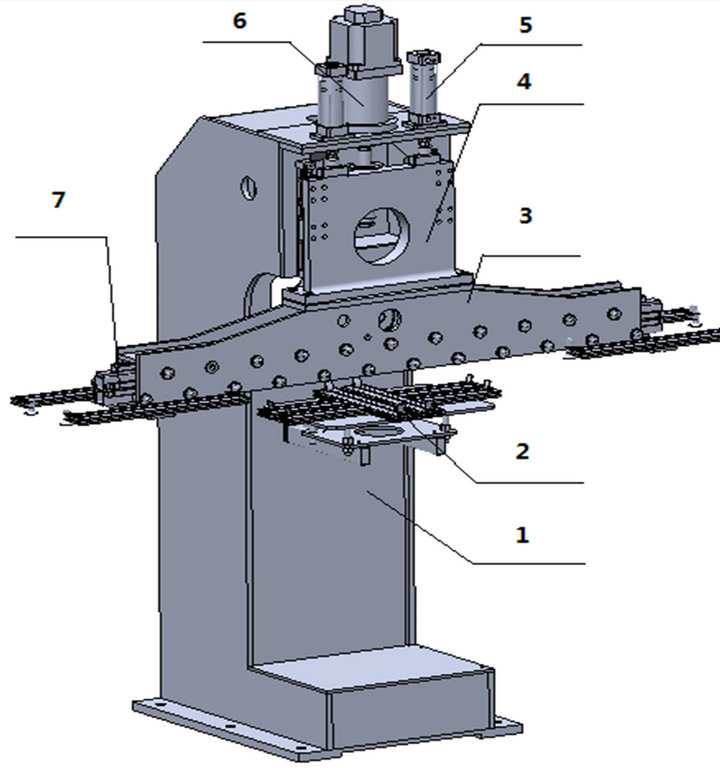
Figure 3. The assembly model of manipulator, 1-body, 2- feeder, 3-beam, 4-slipway, 5-balance cylinder, 6-servo motor, 7-X axis transmission system.
2): Xi axis vertical the axis of Zi and Zi−1 and point to the direction of away from the Zi−1 axis.
3): Yi axis according to the requirements of the right hand coordinate system to establish.
Meanwhile the notation of D-H of the rigid bar depends on the four parameters of the connecting rod.
The angle of two connecting rod ![]() : Xi−1→Xi around the corner of Zi−1.
: Xi−1→Xi around the corner of Zi−1.
The distance of two connecting rod : Xi−1→Xi along the distance of Zi−1.
The length of the connecting rod : Zi−1→Zi along the distance of Xi−1.
The torsion angle of the connecting rod: : Zi−1→Zi around the corner of Xi.
For rotational joints, ![]() is the joint variables, the rest are joint parameters (remain unchanged); for mobile joints,
is the joint variables, the rest are joint parameters (remain unchanged); for mobile joints,  is the joint variables, the rest are joint parameters.
2.2.2. The Design Coordinate of Manipulator
High-speed plate carrying manipulator is mainly composed of vertical pillars (body), horizontal arm (beam), sliding table (Y axis transmission system) and base. Horizontal arm mounted on the machine body level can move around and can move up and down along the vertical pillars. By reference to the high-speed plate carrying manipulator in Figure 3, we establish the coordinate system of manipulator in Figure 4 based on the above analysis.
According to the D-H parameters method, four parameters are defined for each link: the connecting rod angle![]() , the distance of two connecting rod
, the distance of two connecting rod , the length of the connecting rod
 , the connecting rod torsion Angle
 , the D-H parameters of manipulator as is shown in Table 1.
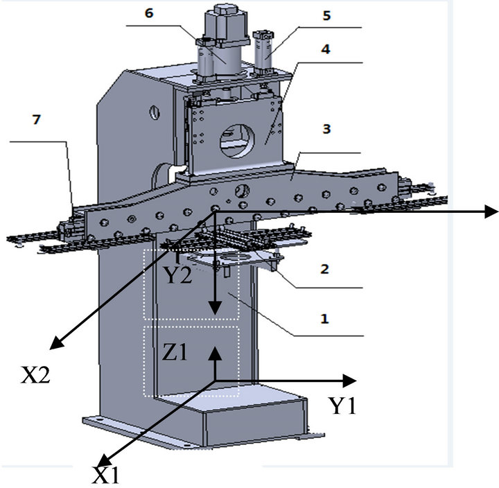
Figure 4. The D-H coordinate of high-speed plate carrying manipulator.

Table 1. The D-H parameters and joint variables of manipulator.
3. The Kinematics Simulation Algorithm of Manipulator
3.1.The Kinematics of Manipulator
The so-called kinematics problem [4,5] is given to the manipulator of each joint variable, and then obtains the position and posture of the end of the actuator, and its essence is to establish the kinematics equations. For the solution of kinematics equation, this paper uses homogeneous transformation matrix ![]() to describe the coordinate system of i relative to the position and pose of the coordinate system of the i – 1, this is the general formula for transformation matrix
to describe the coordinate system of i relative to the position and pose of the coordinate system of the i – 1, this is the general formula for transformation matrix![]() .
.

(1)
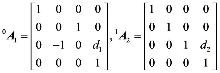
Now, putting the D-H parameters and joint variables of manipulator substitution of the Table 1 in (1), we get the homogeneous transformation matrix of the i coordinate system relative to the position and posture of the base coordinate system, expressed as:
 (2)
(2)
Especially, when ,
,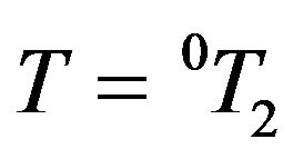 can be obtained, it determines the position and posture of the end of the manipulator relative to the base coordinate system, the matrix of T can be expressed as:
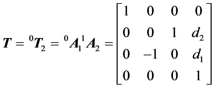 (3)
(3)
Note:
3.2. The Inverse Kinematics Issue of Manipulator
The inverse kinematics issue of manipulator is defined as follows: with the known the position and posture of the end of the actuator, we need to solve the variables of each joint of the manipulator, here in our case the variables are  and
and .
.
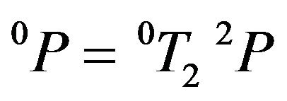
The target point of the movement of the manipulator center is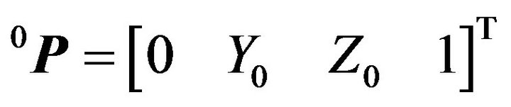 . By using the transitional joint, the manipulator’s center point can coincide with the target point, and the target point can be expressed as:
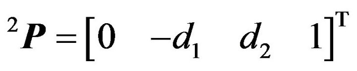 , then we can establish the following equation:
 (4)
(4)
Combining (3) and (4) and solving the kinematics equation , we can get the following equation.
 (5)
(5)
 (6)
(6)
4. The Kinematics Simulation of Manipulator
4.1. Use Link and Robot Functions to Establish the Manipulator’s Object
1) Before the manipulators simulation, firstly input the manipulator’s parameters by calling the function Link:
(note:  represent the variables of
 ,
,  , θi and di respectively; “sigma” represents the joint types: 0 for the rotational joint, and 1 for the transitional joint; “standard” is for the standard D-H parameters. The function robot is used to create a manipulator object by using the Link function in the format of Robot (Link…). The commands for creating the high-speed plate carrying manipulators is expressed as follows:

2) We can immediately see the three-dimensional view of the manipulator which can be used in the form manually for driving through the slider in the chart to drive the movement of the manipulator, which is just like the actual control of the manipulator [3]. As shown in Figure 5, it has brought great convenience for manipulator’s teaching and training.
4.2. The Test of Kinematic Model
In the Figure 5, by moving each slide in the bar to move the manipulator, the first joint movement can change the height of the manipulator in the vertical direction. The second joint can change the length of the manipulator in horizontal direction, So that we can obtain different position and posture. By adjusting the slides and the joint variables, we can get the approximate model corresponding to the actual structure in Figure 3, as shown in Figure 6.
In order to verify the correctness of the kinematics Equation (3), the geometric parameters and the joint variables of each rod of the manipulator are put into the kinematic equations to solve the setting position and posture of the coordinate system of the end link rod in relation to the base coordinate system. And then the corresponding coordinate values are input to the manipulator’s trajectory planning, and the actual end position and posture information are compared with the results from solving the equation. Two groups of joint variable values are randomly chosen :
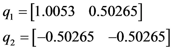
The error is very small through the comparative analysis of the actual value and set point, which explains that the kinematics equation and the model are reliable and consistent.
4.3. The Simulation of Trajectory Planning
According to the requirements of the task, trajectory planning will designate in advance the robot’s operating procedure and action process. The simulation method could describe in details the movement process of the industrial robot [6-10]. Planning can be made in the space of both joint and operation. We would introduce two main motions [4,5]: 1) PTP, Point-To-Point motion; 2) CP, Continuous-Path. With regard to continuous-path, not only the initial and final points of the manipulator need to be set, but also some other points between the two points (called path points) which must move along some specific path (path constraint) need to be indicated.
The design of the high-speed plate carrying manipulator adopts a point-to-point trajectory planning. Set A as the starting point, moving to B where a task is finished, and then set B as a starting point, moving to C where a certain task is completed, and then set C as a starting point, moving to point C to complete the preset tasks, and continue to move, and so on. Here, the move from point A to point B and from point B to point C does not exist any point between them, and there is not any requirement for the known path of the movement. Therefore, we can take this above planning as PTP planning.
The starting point is set to be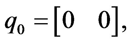 ending point
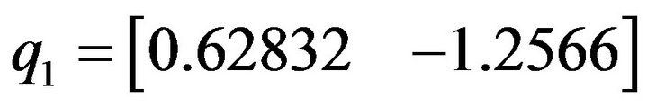 , and between the two
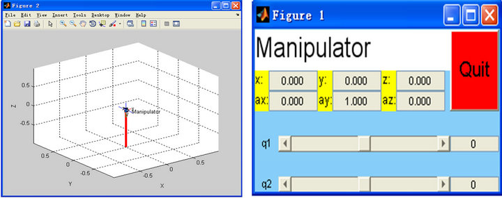
Figure 5. The three-dimensional diagram and slide block control chart of the high-speed plate carrying manipulator.

Figure 6. A state of high-speed plate carrying manipulator’s three-dimensional diagram and slide block control chart.
points the initial and final speeds are both zero, with the time of movement time: , the relative program as follows:
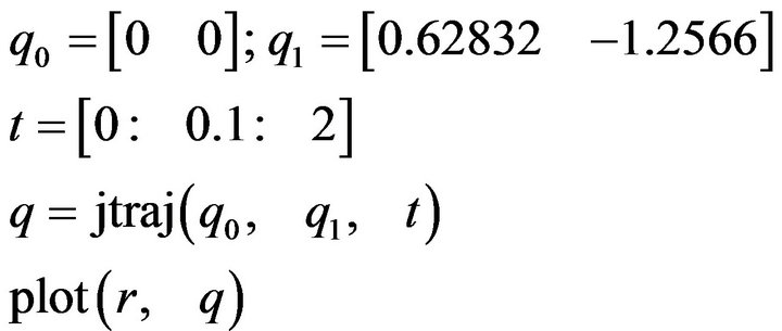
By conducting the above program, we can observe the whole process of the high-speed plate carrying manipulator moving from Figures 5 and 6. We can also draw, by way of the function of

each joint’s displacement curve, as shown in Figure 7(a) and (b). (note: q represents the displacement, i represents the joint Numbers). Also we can draw speed curve as shown in Figures 7(c)-(d), acceleration curve as shown in Figures 7(e)-(f), through the corresponding functions:

4.4. The Analysis Based on the Results of Simulation
From Figures 7(a) and (b), it can be seen that the displacement of the mobile joint 1 gradually changes from zero to 0.62832 m, movable joint 2 displacement from zero change to 1.2566 m; from Figures 7(c) and (d) we

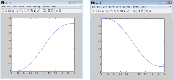

(a) The displacement curve of joint 1 (b) The displacement curve of joint 2
(c)The velocity curve of joint 1 (d) The velocity curve of joint 2
(e) The acceleration curve of joint 1 (f) The acceleration curve of joint 2
Figure 7. Displacement, velocity and acceleration curves of high-speed plate carrying manipulator.
can obtain that the initial and final speeds of the joints 1, 2 are zero, the maximum velocity appearing at the intermediate time t = 1 s; from Figures 7(e)-(f), it can be seen, the initial and final acceleration speeds are zeros, two maximum values in motion, with one positive and the other negative. The manipulator’s displacement curve is smooth, and the curve of velocity and acceleration is continuous. Therefore, it is concluded that: in the process, the manipulator runs smoothly, and the whole body vibrates in a normal scope, which thus explains the validity of the design.
5. Conclusions
The paper carries out a kinematical analysis of a highspeed plate carrying manipulator which is designed by using the module function of Robotics Toolbox in the Matlab. Based on this, we have achieved the following conclusions in three aspects: 1) the structure and parameters of the plate carrying manipulator have been designed; 2) the kinematics model has been established with the standard D-H method, and its positive and inverse kinematics have been analyzed; 3) by using Robotics Toolbox in Matlab, the kinematics model has been set up in order to make the study of the motions of manipulator easier and more apparent, and to conduct a kinematics simulation for the manipulator for obtaining the displacement, velocity and acceleration curve of each manipulator joint. Thus, this proves the validity of the design of manipulator structure parameters, as well as provides the reliable basis for the theoretical analysis in terms of the design, dynamics analysis, and trajectory planning of control system of the manipulator.
REFERENCES
- Q. Wang, X. J. Hu and L. Z. Li, “The Kinematic Analysis and Simulation of the Humanoid Welding Manipulator Based on the MATLAB,” Materials Science and Engineering College of Hefei University of Technology, 2011.
- J. J. Craig, “Introduction to Robotics,” Mechanical Industry Press, Beijing, 2006.
- P. I. Corke, “A Robotics Toolbox for MATLAB,” IEEE Robotics and Automation Magazine, Vol. 3, No. 1, 1996, pp. 24-32. doi:10.1109/100.486658
- X. S. Jiang, “Introduction to Robotics,” Liaoning Science and Technology Press, Shenyang, 1994.
- Z. X. Cai, “The Robotics,” Tsinghua University Press, Beijing, 2000.
- J. X. Luo and G. Q. Hu, “The Kinematic Simulation Research of Robot Based on the MATLAB,” Journal of Xiamen University, JCR Science Edition, Vol. 44, No. 5, 2005, pp. 640-644.
- J. Han and L. Hao, “Trajectory Planning and Simulation of Robot in Joint Coordinate System,” Journal of Nanjing University of Science and Technology, Vol. 24, No. 6, 2000, pp. 540-543.
- Z. X. Wang and W. X. Fan, “The Kinematics Analysis and Simulation of Industrial Robot Based on the Matlab,” Mechanical and Electrical Engineering, Vol. 29, No. 1, 2012, pp. 33-37.
- The MathWorks Inc., “Matlab the Language of Technical Computing Version 6,” The MathWorks Inc., 2002.
- P. I. Corke, “Robotics Toolbox for Matlab (Release 7.1) [EB/OL],” 2002. http://www.cat.csiro.au/cmst/staff/pic/robot