Engineering
Vol. 3 No. 9 (2011) , Article ID: 7327 , 9 pages DOI:10.4236/eng.2011.39108
Application of Geostatistical Models for Estimating Spatial Variability of Rock Depth
1Centre for Disaster Mitigation and Management, VIT University, Vellore, India
2Department of Civil Engineering, Indian Institute of Science, Bangalore, India
E-mail: pijush.phd@gmail.com, sitharam@civil.iisc.ernet.in
Received April 30, 2011; revised May 20, 2011; accepted June 10, 2011
Keywords: Geostatistics, Semivariogram, Kriging
ABSTRACT
Rock depth information of a site is a significant factor for geotechnical engineering and earthquake ground response analysis. In this paper, reduced level of rock at Bangalore is arrived from the 652 boreholes in the area covering 220 km2. Geostatistical modeling based on kriging (simple and ordinary) techniques has been applied for estimating reduced level of hard rock in Bangalore. The models are used to compute variance of estimated reduced level of the rock. A new type of cross-validation analysis proves the robustness of the developed models. The comparison between the simple and ordinary kriging model demonstrates that the ordinary kriging model is superior to simple kriging model in predicting reduced level of rock in the subsurface of Bangalore.
1. Introduction
Rock depth for a site is a very useful parameter to the geotechnical and earthquake engineers to find their basic requirement of hard strata and ground motion at rock level. In most geotechnical investigations, knowledge of the hard strata or hard rock depth is essential to design a suitable foundation. In ground response analysis, Peak Ground Acceleration (PGA) at rock level and response spectrum for the particular site is evaluated. This information is also essential to evaluate liquefaction hazards of a site and to estimate earthquake induced forces on structures.
With an objective of evaluating hard rock depth in Bangalore, an attempt has been made to develop a two dimensional map of reduced level of rock for Bangalore based on kriging (simple and ordinary) technique. Rock is identified by borelogs data available in the area and identified by visual observation of the cores taken at these locations. Hard disintegrated rock is also identified as rock and depth from the ground level has been used to evaluate reduced level of rock at any location.
The kriging method was developed during the 1960s and 1970s and has been acknowledged as a good spatial interpolator [1-3]. The most important features of this method are that the interpolator 1) is linear and unbiased 2) gives minimum estimation error, and 3) is exact and gives an evaluation of uncertainty for interpolated values. This technique is widely used in the field of earth sciences, including mining, geochemistry, remote sensing, etc. A major advantage of kriging is that it is more flexible than other interpolation methods such as inversedistance weighting, deterministic splines and Thiessen polygons. The weights are not selected arbitrarily, but depend on how the variable of interest (in this case hard rock elevation) varies in space. In kriging, the variable weights have been used based on the scale of variability whereas in Thiessen polygon, one has to apply same weights, whether the function exhibits small-or largescale variability. The main goal of kriging is to predict (in the interpolation sense) a variable where no measurements were made using the semivariogram as a model characterizing spatial variability. Semivariogram is the analytical tool used to evaluate and quantify the degree of spatial autocorrelation. It contains three elements of information. First of all the semivariogram is an appreciation of the dispersion (or scatter) of the parameters, which equates to the half variance. Secondly, it gives an autocorrelation distance that represents the radius of influence of a measurement made at a given point. Thirdly, it provides the type of variability that indicates how values fluctuate in space.
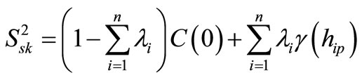
A valid estimation of the variance of estimated reduced level of rock depths is important for developed ordinary as well as simple kriging model. So, the developed models have been used to compute variance of estimated reduced level of the rock depths. In general, the variance depends both on the semivariogram and the location of the measurements. A number of publications can be found in the literature which presents the theory and application of kriging [4-12].
In this paper, a semivariogram model has been developed along with the kriging model for the reduced level of the rock in the subsurface of Bangalore. Semivariogram analysis is used to detect trends in structure or internal properties of deposits and estimated values can be obtained at points where no data is available. A new method for cross-validation analysis of developed models has been proposed. The cross-validation of the model has been done based on the examination of residuals. A comparative study has been also done between developed simple kriging and ordinary kriging.
2. Subsurface of Bangalore and GIS Model Development
Bangalore covers an area of over 220 square kilometres and ground Reduced levels (GRL) also vary a lot in the city. It varies from 810 m in north-east part to 940 m in south-western part of Bangalore. Ground reduced levels do not vary much in the central and north-western parts of the city. The population of greater Bangalore exceeds 6 million and it is the fifth biggest city in India. It is situated on latitude of 1208' North and longitude of 77037' East. From geology, subsurface of Bangalore region is a Gneiss complex, which was formed by several tectonic-thermal events with large influx of sialic material, occurring between 3 to 3.4 billion years ago giving rise to an extensive group of gray gneisses designated as the “older gneiss complex”. These gneisses act as the basement for a widespread belt of schist’s. The younger group of gneissic rocks mostly of granodiomitic and granitia composition is found in the eastern part of the state, representing remobilized parts of an older crust with abundant additions of newer granite material, for which the name “younger gneiss complex” has been given [13]. The soil is mostly a residual soil from granite gneiss due to weathering action. In the most recent past, there were more than 400 lakes, and more than 340 lakes were dried up and have been encroached for residential and industrial development. In the old tank beds, silty sand/clay is also found as overburden.
A Geographic Information System (GIS) model (see Figure 1) of Bangalore with several layers on a scale of 1:20,000 has been developed with a purpose of carrying out microzonation of Bangalore. The Bangalore map forms the base layer for GIS. The map entities have been developed for locating boreholes to the utmost accuracy and at each location borelogs have been attached along with geotechnical data of each layer up to the hard rock. The digitized map has several layers of information. Some of the important layers considered are the boundaries (outer and Administrative), Highways, Major roads, Minor roads, Streets, Rail roads, Water bodies, Drains, Ground Contours and Borehole locations. The locations of boreholes are shown in Figure 1 along with ground reduced level with an interval of 10 m (see Figure 2). Distribution of collected boreholes in Bangalore is shown in Figure 3, indicating a very good distribution of the boreholes in each quadrant of Bangalore from the city center. Figure 1 also depicts grids of 1kmΧ1km along with the corporate boundary of Bangalore and outer boundary circumscribing the ring road. Figure 1 gives a clear view of the spatial distribution of boreholes in Bangalore region. An average of about three boreholes data is available within the grid of 1 km × 1 km.
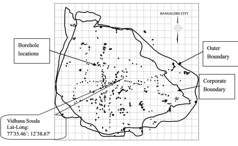
Figure 1. Borehole location in Bangalore Map (scale: 1:20000).
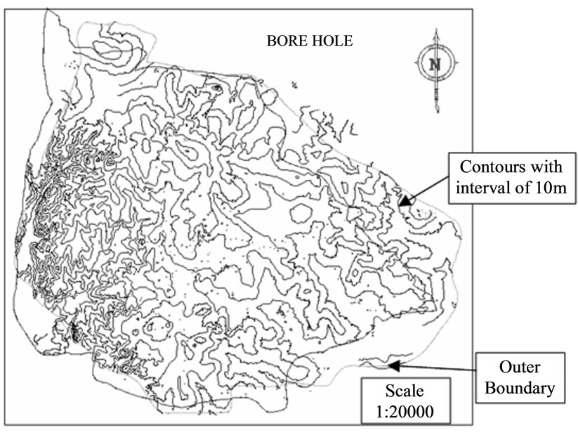
Figure 2. GIS model of borehole locations with respect to contours.
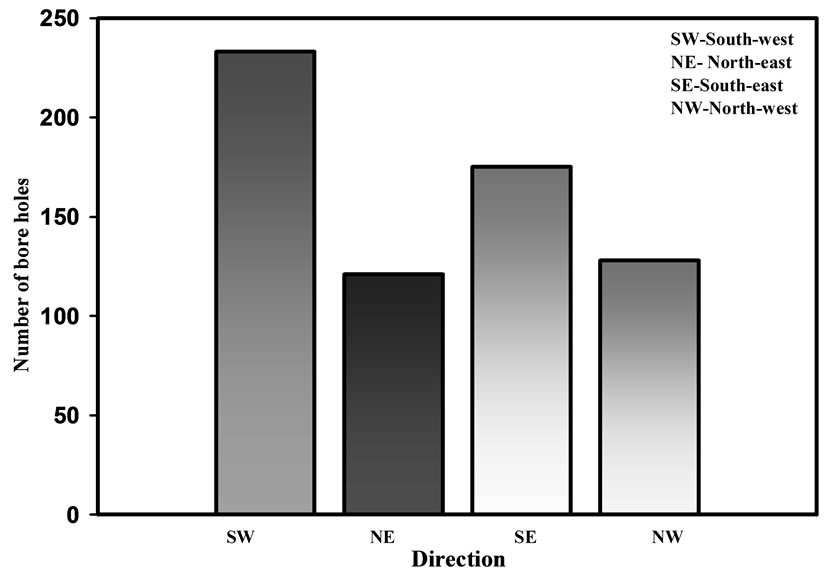
Figure 3. Distribution of boreholes in quadrants of Bangalore.
Geotechnical data for 652 boreholes was collated from archives of only two organizations; Torsteel Research Foundation in India and Indian Institute of Science. This data was generated for geotechnical investigations carried out for several major projects in Bangalore including Bangalore metro project. The data collected is of very high quality and collected during the years 1995-2003. The data in the model is on average to a depth of 30m below the ground level. Each borelog contains information about depth, density of the soil, total stress, effective stress, fines content and N values, depth of ground water table and rock depth. In GIS model, the boreholes are represented as three dimensional object spanning below the map layer. These three dimensional objects are generated with several layers with a bore location in each layer overlapping one below the other and each layer representing 0.5m interval of the subsurface. Each layer of this model is attached with borelog data at that depth. The data consists of visual soil classification, borehole location, ground water level, date and time during which test has been carried out, other physical and engineering properties of soil and rock depth. As such when this model is viewed in three dimensions, subsurface information on any borehole at any depth can obtained by clicking at that level. The hard rock has been identified by visual observation of the cores taken at these locations. Rock depth from ground level is the difference between the ground reduced level at borehole location and reduced level of the hard rock at the same borehole location. The reduced level of the hard rock at borehole location is the difference between the ground reduced level at borehole location and depth of overburden thickness up to hard rock in the same borehole. The depth of overburden is estimated from the available borelogs. The term hard rock in this paper corresponds to engineering bed rock (shear wave velocity ≈700 m/sec) as against seismic bed rock (shear wave velocity ≈3000 m/sec).
3. Methodology
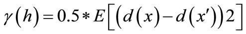
In this paper, ordinary kriging and simple kriging are adopted for evaluating reduced level of the rock in subsurface of the Bangalore. For both the methods, there is a need to introduce the terminology of the covariance function or semivariogram. The covariance function between two points is defined as:
 (1)
(1)
where m is the mean of d(x) and C(h) is the covariance function with lag h, with h being the distance between two samples x and x':
 (2)
(2)
The semivariogram for an intrinsic random function [14,15] is defined as:
 (3)
(3)
Figure 4 illustrates the different components of the semivariogram.
If the variance exists (the random function is second order stationary), the relation between the covariance function and the semivariogram is as follows:
 (4)
(4)
where,  is the semivariogram and
  is the variance.
For semivariogram, the model used in this analysis is Gaussian model. The general equation for this model looks like:
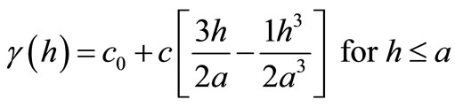 (5)
(5)
 (6)
(6)

Figure 4. A typical semivariogram.
For semivariogram model, geoanisotropic model has been used to reduce the anisotropy into isotropy by a linear transformation of coordinates [16]. Once the model of semivariogram is constructed, the weights are computed for kriging. The method for ordinary kriging, simple kriging and cross-validation of the models are given as below:
3.1. Ordinary Kriging
Ordinary kriging is a linear geostatistical method. It gives local estimation by interpolation. The basic equation used in ordinary kriging is as follows:
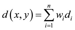 (7)
(7)
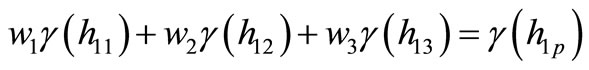
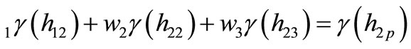
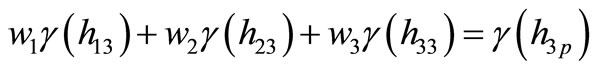
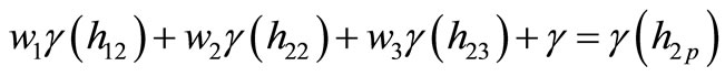
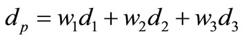
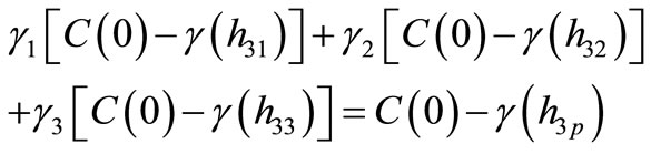
where n is the number of scatter points in the subsurface of the Bangalore. di is reduced level of the rock at point i in the subsurface of the Bangalore and wi is weights assigned for point i. This equation is essentially the same as the equation used for inverse distance weighted interpolation except that rather than using weights based on an arbitrary function of distance. The weights used in kriging are based on the model semivariogram. For example, to interpolate reduced level of the rock (dP), at a point ‘P’ in the subsurface of the Bangalore based on the surrounding points P1, P2, and P3, the weights w1, w2, and w3 must be found. The weights are found through the solution of the simultaneous equations:
 (8)
(8)
 (9)
(9)
 (10)
(10)
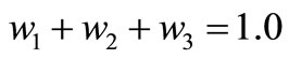
where (hij) is the model semivariogram evaluated at a distance equal to the distance between points i and j in the subsurface of the Bangalore. For example (h1p) is the model semivariogram evaluated at a distance equal to the separation of points P1 and P. Since it is necessary that the weights sum to unity, a fourth equation is added.
 (11)
(11)
Since there are now four equations and three unknowns, a slack variable, is added to the equation set. The final set of equations is as follows:
 (12)
(12)
 (13)
(13)
 (14)
(14)
 (15)
(15)
The equations are then solved for the weights w1, w2, and w3. The dp value of the point p is then calculated as:
 (16)
(16)
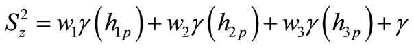
where, d1, d2 and d3 are reduced level of the rock at point P1, P2 and P3 respectively. The variance can be calculated at each interpolation point as:
 (17)
(17)
when interpolating to an object using the kriging method, variance data set is always produced along with the interpolated data set. In some cases, specific spatial data distributions give rise to negative kriging weights, causing interpolated values to be negative or out of data limits and physically not compatible with data. For this reason negative and particular positive weights are set to 0 according to the rules proposed by Deutsh [17], ensuring the sum of weights is equal to one.
3.2. Simple Kriging
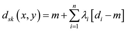
Simple kriging uses the average of the entire data set. The basic equation used in simple kriging is as follows:
 (18)
(18)
where  is weight assigned for point i and m is the average value.
The weights  are found through the solution of the simultaneous equations:
 (19)
(19)
 (20)
(20)
 (21)
(21)
The variance of estimation then become equal to
 (22)
(22)
3.3. Cross-Validation of the Models
A new type of cross-validation analysis for kriging has been presented in this study. In practice, cross-validation is based on statistical tests involving the residuals. Residuals are differences between observation and model predictions. The detailed description of residuals in the case of kriging is given by Kitanidis [16]. It has been assumed that the n measurements are available at a time, in a given sequence. The kriging estimate of z at the second point, x2 from the first measurement, x1 is calculated. So, one can write  and
and  . Where,
  is the kriged value at the point x2. The actual error
  is normalized by the standard error (
 ) and this normalized value of the error is given by:
 (23)
(23)
For the k-th measurement location, the actual error (δk) and normalized error  can be written as, respectively:
 (24)
(24)
 (25)
(25)
A cross-validation Q1 and Q2 are used to check the statistical distribution of the residuals between the observed data and kriged values at the original observation location by using the same kriging parameters and semivariogram model parameters. To perform Q1 and Q2 cross validation, a normalized residual array (εk) is constructed as suggested by Kitanidis (1997). Q1 is the mean of the residual (εk) and it is written as:
 (26)
(26)
Under the null hypothesis, Q1 is normally distributed with mean 0 and variance . The probability density function (pdf) of Q1 is:
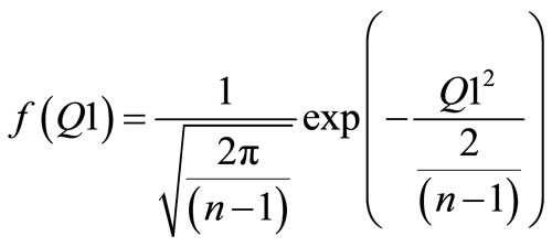 (27)
(27)
where, n is the number of data points. If the experimental value of Q1 turns out to be acceptable close to zero then this test gives no reason to question the validity of the model. The Q2 is the variance of εk and it is written as:
 (28)
(28)
 approximately follows the chi-square distribution with parameter
 . Where, n is the number of data points. The mean and variance of Q2 are 1 and
  respectively. The pdf of Q2 is given by the following equation:
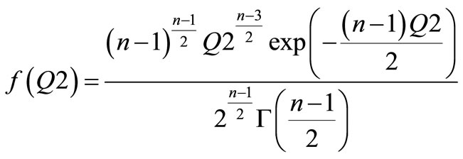 (29)
(29)
where, G is the gamma function. For robust model, the experimental value of Q2 should be close to one. In this work, kriging model and cross-validation have been programmed using MATLAB software.
4. Results and Discussion
In case of ordinary kriging, the semivariogram of reduced level of rock obtained from the experimental values is shown in Figure 5. The Gaussian model has been plotted in Figure 5 and gives a reasonable fit to the values obtained. The range, sill and nugget of the semivariogram are 0.95, 1.202 and 0.097 respectively. In the semivariogram, on the x-axis “relative to the full length scale” means normalized lag distance. The estimation of reduced level of rock has been done by using developed model of semivariogram (shown in Figure 5). Figure 6 shows the kriging surface of the reduced level of rock for ordinary kriging. For simple kriging analysis, the experimental semivariogram has been calculated using the reduced level of rock data. A Gaussian model has been fitted with parameters: 0.95 for range, 1.178 for sill and 0.079 for nugget. By using the model of the semivariogram shown in Figure 7, reduced level of rock has been estimated in the subsurface of the Bangalore. The result is shown in Figure 8.
One of the most important finding of this study is that the semivariogram for both models is free from white noise or a pure nugget effect. The pure nugget effect corresponds to the total absence of auto-correlation. A weighted nonlinear least squares method has been used to fit semivariogram model. The points closer to the origin are given higher weights than points further away, because they are inherently more accurate, as they are calculated using more data pairs. Gaussian model, which has been used for semivariogram, ensures well-conditioned
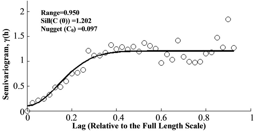
Figure 5. Semivariogram model using ordinary kriging.
kriging matrix. So this study did not exhibit any numerical stability problem. For both models, the semivariogram stops increasing beyond a certain distance. This semivariogram is called “transition” models, and corresponds to a random function which is not only intrinsic but also stationary. A function is stationary if it consists of small scale fluctuations about some well-defined mean value. For a stationary function, the length scale at which the sill is obtained describes the scale at which two measurements of the variable become practically uncorrelated. The advantage of intrinsic model is that it has been used to summarize incomplete information and patterns in noisy data. It has been also used to interpolate unknown data from observation of data. The semivariogram has a sill, which indicates that having extreme values has a very low probability. The both kriging models gave a unique solution. The reason for unique solution is explained below.
Considering a case of two different measurements of reduced level of rock obtained at the same location, if the semivariogram for both models is continuous (with zero nugget) the function d(x) will be continuous. This means that one of the two measurements is redundant. Thus, one must be discarded; otherwise, a unique solution cannot be obtained because the determinant of the matrix coefficients of the kriging system vanishes. This problem is solved by adding a nugget term to the semivariogram. As a result, the Gaussian model adopted shows the nugget effect. In practical sense, nugget effect gives the kriging equations a stability and robustness. Without a nugget effect, inverting the kriging matrices may lead to computational round-off errors. Nugget effect also confirms that the contour map of estimate has a discontinuity at each observation point. As the sampling distance decreases, it is possible to obtain a better estimate of nugget effect. But the cost of the exploration program increases enormously. The model for the experimental semivariogram has been chosen based on the examination of residuals (differences between observation and model predictions). The predicted values from simple and ordinary kriging are different because of their different properties. As a result, the residuals from simple and ordinary kriging are different. For this reason, the semivariograms are different for simple and ordinary kriging. In this study, the residuals are always uncorrelated. The lack of correlation in the residuals has been explained below:
If the residuals are correlated, one can use this correlation to predict the value of  from the value of
  using a linear estimator. So, one can reduce further the mean square error of estimation of d(xk). But this is impossible because d(xk) is already the minimum-variance estimate. Thus, the residuals must be uncorrelated.
Kriging maps (Figures 6 and 8) provide a qualitative difference between the ordinary kriging and simple kriging methods. The advantage of this study is that it provides the magnitude of the variance of the estimated reduced level of rock. Figure 9 is the variance map of reduced level of rock generated by ordinary kriging. Figure 10 is a variance map of reduced level of rock generated by simple kriging. Using kriging variance map (Figures 9 and 10), one can give an indication of the quality of estimate. From Figures 9 and 10, it has been seen that the variance increases with increasing distance between estimated points and the actual point. The overall pattern of Figures 9 and 10 give an indication of where in the field adequate or inadequate sampling occurred. In the Figures 9 and 10, it is clear that the variance of the estimated data from simple kriging analysis is
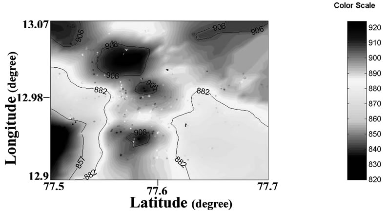
Figure 6. Map of the reduced level of rock for Bangalore using ordinary kriging.
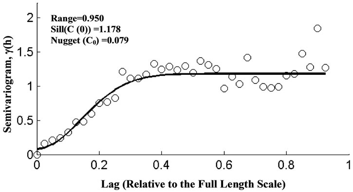
Figure 7. Semivariogram model using simple kriging.
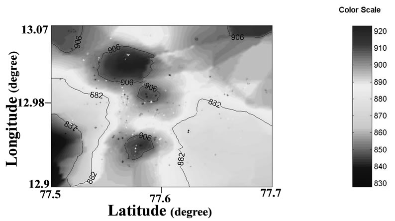
Figure 8. Map of the reduced level of rock for Bangalore using simple kriging.

Figure 9. Map of the variance of the estimated reduced level of rock for Bangalore using ordinary kriging.
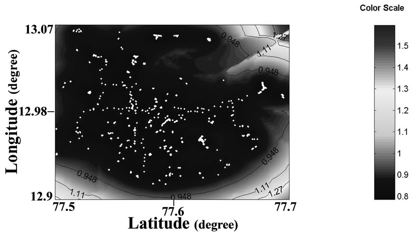
Figure 10. Map of the variance of the estimated reduced level of rock for Bangalore using simple kriging.
always greater than the variance of the estimated data from ordinary kriging analysis. Prediction of variance also depends on the behavior of the semivariogram at the origin, and it is known that without a nugget effect the predicted variance is often underestimated.
In case of cross-validation of kriging model, the acceptable region is defined in the Figures 11 to 14 (between the two vertical lines). For a good model, the Q1 as well as Q2 must fall in this acceptable regions as shown in Figures 11-14. In case of ordinary kriging, the value of Q1 and Q2 is 0.002, 1.069 respectively. The Q1 and Q2 values are well within the acceptable region (shown in Figures 11 and 12). In case of simple kriging, the value of Q1 and Q2 is 0.01, 0.911 respectively. The Q1 and Q2 fall in the acceptable region (shown in Figures 13 and 14). For both the models, the value of Q1 and Q2 are close to 0 and 1 respectively. The crossvalidation indicates that the developed ordinary kriging as well as simple kriging models are robust models for the estimation of the reduced level of rock in the subsurface of Bangalore. However it is clear from the results that the ordinary kriging seems to be predicting better than simple kriging.
In order to compare between the ordinary and simple kriging models, five points have been chosen randomly from known reduced level of the rock of 652 points in
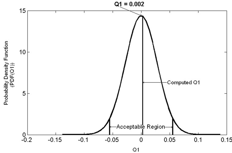
Figure 11. Distribution of Q1 for ordinary kriging.

Figure 12. Distribution of Q2 for ordinary kriging.
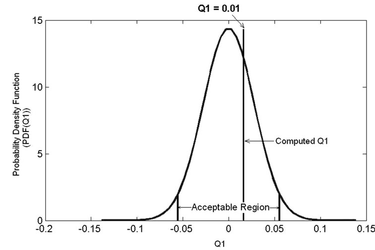
Figure 13. Distribution of Q1 for simple kriging.

Figure 14. Distribution of Q2 for simple kriging.
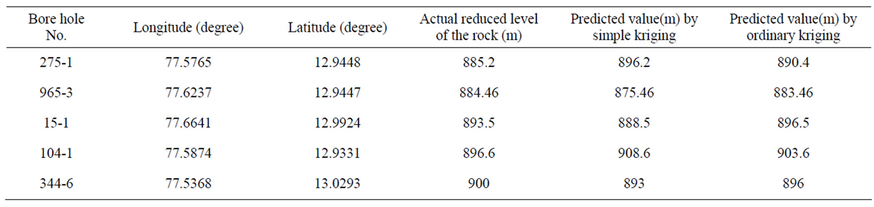
Table 1. Comparison between ordinary kriging and simple kriging model.
the subsurface model of Bangalore. The predicted values of these points are shown in Table 1. It can be seen from the table that the ordinary kriging model has given better prediction than simple kriging model. For the data sets used in this paper, ordinary kriging has shown to be a better estimator than simple kriging in terms of reduced kriging variance and the comparison between an estimated and actual value. This result is expected, since the simple kriging uses the average of the entire data set while ordinary kriging uses a local average (the average of the scatter points in the kriging subset for a particular interpolation point). The reduced level of rock at a half-space point could be more accurately estimated from the reduced level of rock at neighboring half-space points than that at distinct location. As a result, simple kriging is less accurate than ordinary kriging.
First, confirm that you have the correct template for your paper size. This template has been tailored for output on the A4 paper size. If you are using US letter-sized paper, please close this file and download the file for “MSW US ltr format”.
Maintaining the Integrity of the Specifications
The template is used to format your paper and style the text. All margins, column widths, line spaces, and text fonts are prescribed; please do not alter them. You may note peculiarities. For example, the head margin in this
5. Conclusions
This study has demonstrated the usefulness of kriging as a tool to determine the reduced level of the rock in Bangalore considering a large data set (652 points) distributed over 220 sq·km area. Geostatistics has permitted the development of a semivariogram model for predicting reduced level of the rock in Bangalore.
The power of geostatistics has become even more apparent through the estimated reduced level of the rock in a way that is consistent with what we know from the field data. By the use of semivariogram, it is possible to make estimation of the reduced level of the rock at points of the site where reduced levels of the rock were not known. The models have been developed by using simple as well as ordinary kriging methods. Variance map for both kriging techniques have been generated and presented. A new type of cross-validation analysis (Q1 and Q2) which proves the robustness of the developed kriging models has been also presented in this study. Ordinary kriging yielded better results than simple kriging for estimation of reduced level of the rock in the subsurface of Bangalore.
6. REFERENCES
- G. Matheron, “Principles of Geostatistics,” Society of Economic Geologists, Vol. 58, No. 8, 1963, pp. 1246- 1266. doi:10.2113/gsecongeo.58.8.1246
- E. H. Isaaks and R. M. Srivastava, “An Introduction to Applied Geostatics,” Oxford University Press, New York, 1989.
- J. C. Davis, “Statistics and Data Analysis in Geology,” 3rd Edition, Wiley, New York, 2002.
- J. P. Delhomme, “Spatial Variability and Uncertainty in Groundwater Flow Parameters: A Geostatistical Approach,” Water Resources Research, Vol. 15, No. 2, 1979, pp. 269-280. doi:10.1029/WR015i002p00269
- F. Gambolati and G. Volpi, “Groundwater Contour Mapping in Venic by Stochastic Interpolators 1. Theroy”. Water Resources Research, Vol. 15, No. 2, 1979, pp. 281-290. doi:10.1029/WR015i002p00281
- M. Soulie, “Geostatistical Applications in Goetechnics,” Geostatistics for Naturai Resources Characterization: Part 2, NATO ASI Series,” Reidel Publishing Company, Dordrecht, 1983, pp. 703-730.
- P. H. S. W. Kulatilake and A. Ghosh, “An Investigation into Accuracy of Sparial Variation Estimation Using Static Cone Penetrometer Data,” Proceeding of the First Internatioanl Symposium on Penetration Testing, Orlando, 1988, pp. 815-821.
- P. H. S. W. Kulatilake, “Probabilistic Potentiometric Surface Mapping,” Journal of Geotechnical & Geoenvironmental Engineering, Vol. 115, No. 11, 1989, pp. 1569-1587. doi:10.1061/(ASCE)0733-9410(1989)115:11(1569)
- M. Soulie, P. Montes and V. Sivestri, “Modeling Spatial Variability of Soil Parameters,” Canadian Geotechnical Journal, Vol. 27, No. 5, 1990, pp. 617-630. doi:10.1139/t90-076
- P. Chiasson, J. Lafleur, M. Soulie and K. T. Law, “Characterizing Spatial Variability of Clay by Geostatistics,” Canadian Geotechnical Journal, Vol. 32, No. 1, 1995, pp. 1-10. doi:10.1139/t95-001
- M. W. O’Neill and L. M. Yoon, “Spatial Variability of CPT Parameters at University of Houston NGES,” Probabilistic Site Characterization at the National Geotechnical Experimental Sites, Geotechnical Special Publication, Vol. 121, 2004, pp.1-12.
- K. M. Dawson and L. G. Baise, “Three-Dimensional Liquefaction Potential Analysis Using Geostatistical Interpolation,” Soil Dynamics and Earthquake Engineering, Vol. 52, No. 5, 2005, pp. 369-381. doi:10.1016/j.soildyn.2005.02.008
- B. P. Radhakrishna and R. Vaidyanadhan. “Geology of Karnataka,” Geological Society of India, Bangalore, 1997.
- G. Matheron,“Théorie des Variables Régionalisées in Traité d’Informatique Géologique,” Masson, Paris, 1972, pp. 306-378.
- A. Guillaume, “Introduction a la Géologie Quantitative,” Masson, Paris, 1977.
- P. K. Kitanidis, “Introduction to Geostatistics: Applications in Hydrogeology,” University Press, Cambridge, 1997, pp. 86-95.
- C. V. Deutsh, “Correcting for Negative Weights in Ordinary Kriging,” Computers & Geosciences, Vol. 22, No. 7, 1996, pp. 765-773. doi:10.1016/0098-3004(96)00005-2