Engineering
Vol. 3 No. 3 (2011) , Article ID: 4142 , 4 pages DOI:10.4236/eng.2011.33025
Developing Intensity-Duration-Frequency Curves in Scarce Data Region: An Approach Using Regional Analysis and Satellite Data
1Civil Department, Fayoum University, Al Fayoum, Egypt
2Civil Department, Cairo University, Giza, Egypt,
3Civil Department, Ain Shams University, Cairo, Egypt
E-mail: aawadallah@darcairo.com
Received December 21, 2010; revised January 11, 2011; accepted February 9, 2011
Keywords: Rainfall Frequency Analysis, Regional Analysis, Intensity Duration Frequency, TRMM, Angola
ABSTRACT
The availability of data is an important aspect in frequency analysis. This paper explores the joint use of limited data from ground rainfall stations and TRMM data to develop Intensity Duration Frequency (IDF) curves, where very limited ground station rainfall records are available. Homogeneity of the means and variances are first checked for both types of data. The study zone is assumed to be belonging to the same region and checked using the Wiltshire test. An Index Flood procedure is adopted to generate the theoretical regional distribution equation. Rainfall depths at various return periods are calculated for all stations and plotted spatially. Regional patterns are identified and discussed. TRMM data are used to develop ratios between 24-hr rainfall depth and shorter duration depths. The regional patterns along with the developed ratios are used to develop regional IDF curves. The methodology is applied on a region in the North-West of Angola.
1. Introduction and Methodology
The availability of data is an important aspect in frequency analysis. The estimation of probability of occurrence of extreme rainfall is an extrapolation based on limited data. Thus the larger the database, the more accurate the estimates will be. From a statistical point of view, estimation from small samples may give unreasonable or physically unrealistic parameter estimates, especially for distributions with a large number of parameters (three or more). Large variations associated with small sample sizes cause the estimates to be unrealistic. In practice, however, data may be limited or in some cases may not be available for a site. In such cases, regional analysis is most useful.
The main objective of this paper is to present the methodology and results aiming at developing intensityduration-frequency (IDF) curves in a region where ground rainfall stations data is scarce. To complement the data, Tropical Rainfall Measuring Mission (TRMM) corrected satellite data was used. TRMM is a joint U.S.-Japan satellite mission to monitor tropical and subtropical (40˚ S–40˚ N) precipitation. TRMM satellite data are available from 1998 to 2008. Several studies have compared the TRMM data with ground station data ([1-4]); however, the aim of this study is to explore the joint use of TRMM data with ground station data to produce intensity-duration-frequency relations.
The first step is to assess if the TRMM annual maximum daily data have different average (compa-red to ground station data) using the Mann-Whitney U, the Moses extreme reactions, the Kolmogorov-Smirnov Z, the Wald-Wolfowitz runs tests. Furthermore, the Levene test was performed to check the equality of variance between the two data types.
Once the possibility of the joint use of maximum daily rainfall from ground stations and TRMM data is checked, the combined maximum daily records at locations of interest are verified if they belong to the same region via the Wiltshire test and the ordinary moment diagram. An Index Flood method is then applied to get the regional estimates of the maximum daily rainfall at different return periods.
The regional estimates are first compared with the at-site estimates, and the ones that better fit the raw data are selected. Subsequently, the adopted estimates for all locations are compared in order to establish geographically coherent regions. Since the main purpose is to develop intensity-duration-frequency curves, the lower (less conservative) values that might appear in certain locations and that are not consistent with the geographically coherent region are discarded.
Following the establishment of the geographically coherent regional average estimates of the daily rainfall at different return periods, the ratios between intensities of the 24-hr and those of the 12-, 6-, 3-, 2-, 1-Hr, 30-, 15-, and 5-min based on Bell [5] and SCS type II dimensionless rainfall curve [6] are used to derive the short duration rainfall values of the IDF. As such, regional robust IDFs are developed for scarce data regions.
The application of the methodology is in a region of North-West Angola where IDF curves are needed for eight cities; namely, Sazaire (Soyo), Ambriz, Quinzau, Landana, Noqui, Maquela do Zombo, M Banza Congo, and Cuimba, shown on Figure 1. Maximum annual rainfall data coming from ground rainfall stations for the eight cities are only available for 8 years at most.
The paper is organized as follows. After the current section presenting the paper objective, its methodology and region of application, the rainfall data available from the ground stations and TRMM are described. The following section presents the results of homogeneity tests verifying the possibility of the joint use of ground data and TRMM. The regionalization methodology is detailed in the fourth section illustrating the Wiltshire test and the index flood method. The results of the regionalization are illustrated in the subsequent section followed by the assumptions of the IDF development. Finally, conclusions are offered in the last section.
2. Rainfall Data Available for Ground Stations and TRMM
In the procedure of developing the Intensity Duration
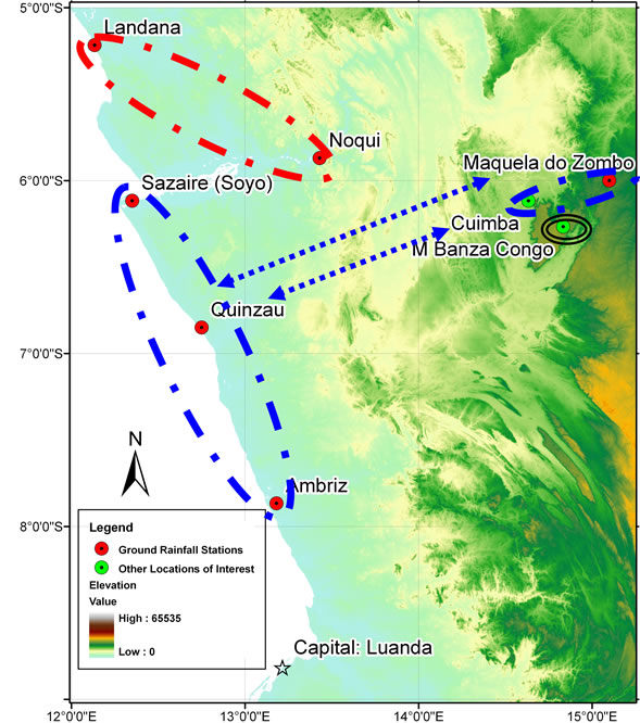
Figure 1. Rainfall stations that will be used during the analysis.
Frequency (IDF) curves for the North-West of Angola, the data was collected from the ground rain gauging stations. The following Table 1 shows the names and coordinates of ground rainfall stations used in this study. Figure 1 shows these stations along with other locations of interest for which an IDF is required, on the Shuttle Radar Topography Mission (SRTM) elevation data (90 m resolution at ground) in the background. SRTM data is obtained on a near-global scale to generate the most complete high-resolution digital topographic database of Earth. It consisted of a modified radar system that flew onboard the Space Shuttle Endeavour during an 11-day mission in February of 2000.
Unfortunately, recent ground stations records were not available. Old data were retrieved from the National Oceanic and Atmospheric Agency in the USA, which keeps in its data rescue website, scanned reports of “Elementos Meteorológicos e Climatológicos” of the “Serviços de Marinha, Repartição Técnica de Estatística Geral”. The reports available on the NOAA website cover the period from 1943 to 1952. However, some stations were not functioning properly even during this short period. Table 2 shows the maximum daily rainfall depth recorded for each ground station in millimeter.
As limited data are available, Tropical Rainfall Measuring Mission (TRMM) data was used. TRMM data give rainfall depths every 3 hours and are downloadable from http://disc2.nascom.nasa.gov/Giova-nni/tovas/site. Table 3 shows the maximum daily rainfall depth recorded for each location of interest in millimeter.
3. Homogeneity Check
The frequency analysis of rainfall data records is affected by the number of records for each station; therefore carrying the analysis for all the records available shall give higher confidence to the results.
However, the TRMM data should be tested first if they can be combined to the ground data in one set. Several tests are available to test the homogeneity of the mean and the variance. This is described in the below sub-sections.
3.1. Homogeneity of the Mean
To test the homogeneity of the mean, several non parametric tests [7] are available, among them the MannWhitney U [8] and Wilcoxon W [9] tests which are equivalent. Non-parametric tests are preferred as the data dealt with are known a-priori to be non-normal. In the following we present the procedure of the Mann-Whitney test as a representative of the applied test and we present the results of both tests. Both of them confirm that there is no statistical evidenceto a 5% level of significance — that there is a significant difference in the mean of the two samples (Table 4).
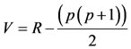
In this test, two samples of size p and q are compared. The combined dataset of size N = p + q is ranked in increasing order. The Mann-Whitney (M-W) test considers the quantities V and W in Equations (1) and (2)
 (1)
(1)
 (2)
(2)
R is the sum of the ranks of the elements of the first sample (size p) in the combined series (size N), and V and W are calculated from R, p, and q. V represents the number of times an item in sample 1 follows an item in sample 2 in the ranking. Similarly, W can be computed for sample 2 following sample 1. The M-W statistic U is defined by the smaller of V and W.
Other non-parametric tests such as the Moses extreme reactions [10], the Kolmogorov-Smirnov Z, the WaldWolfowitz runs tests [11] are reported in Tables 5 to 7. They all confirm that there is no statistical evidence-to a 5% level of significance-that there is a significant difference in the mean of the two samples. For details about these tests, the reader is referred to [7].
3.2. Homogeneity of the Variance
Levene’s test [12] is an inferential statistic used to assess the equality of variance in different samples. Levene’s test assesses that variances of the populations, from which different samples are drawn, are equal. It tests the null hypothesis that the population variances are equal. If the resulting p-value of Levene’s test is less than some critical value (typically .05), the obtained differences in sample variances are unlikely to have occurred based on random sampling. Thus, the null hypothesis of equal variances is rejected and it is concluded that there is a difference between the variances in the population. One advantage of Levene’s test is that it does not require
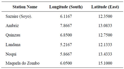
Table 1. Ground rainfall gauges coordinates.
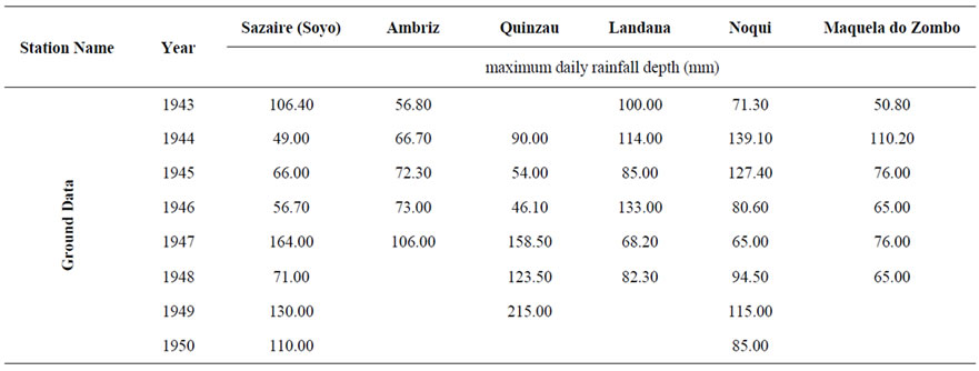
Table 2. Maximum daily rainfall depths based on ground rainfall gauges.
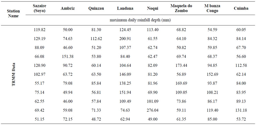
Table 3. TRMM maximum daily rainfall depth recorded in years 1998 to 2008 for locations of interest.
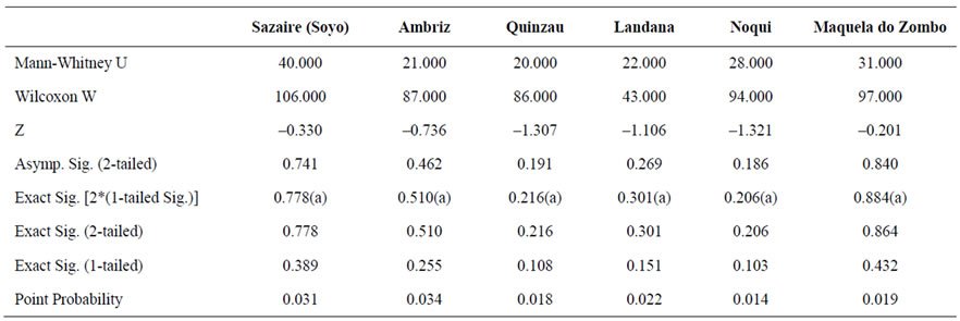
Table 4. Mann-whitney U and wilcoxon W statistics.
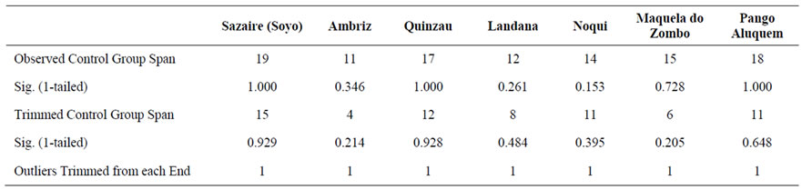
Table 5. Moses test statistics.
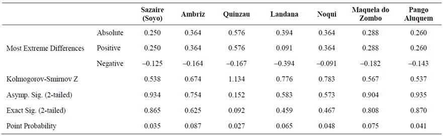
Table 6. Kolmogorov-smirnov test statistics.
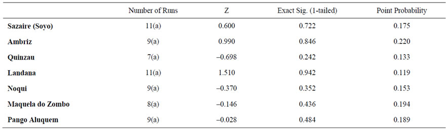
Table 7. Wald-wolfowitz test statistics.
normality of the underlying data. The application of Levene test (Table 8) shows that for all stations (except Quinzau) the variance of the ground data is not statistically significant (at 5% level of significance) from the variance of the TRMM data. Since a regionalization procedure will be used to undertake the frequency analysis, the variance of a single station is not a governing factor in the global regional analysis.
4. Regionalization Methodology
Regionalization serves two purposes. For sites where data are not available, the analysis is based on regional data [13]. For sites with available data, the joint use of data measured at a site, called at-site data, and regional data from a number of stations in a region provides sufficient information to enable a probability distribution to be used with greater reliability. This type of analysis represents a substitution of space for time where data from different locations in a region are used to compensate for short records at a single site [14] and [15].
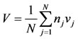
Regional frequency analysis methods are based on the assumption that the standardized variable qt = QT/μi at each station (i) has the same distribution at every site in the region under consideration, where QT is the quantile at t return period and μi is the mean of the maximum daily rainfall record at location i. In particular Cv(q) and Cs(q), the coefficient of variation and the coefficient of

Table 8. Independent samples Levene test.
skewness of q, are considered to be constant across the region [13]. Departures from this assumption may lead to biased quantile estimates at some sites. Sites with Cv and Cs nearest to the regional average may not suffer from such bias, but large, biased quantile estimates are expected for sites whose Cv and Cs deviate from average. Good results may be obtained by regionalization, especially in cases of short records, provided that the degree of heterogeneity is not great. In such cases, the large number of sites contributing to parameter estimation compensates for regional heterogeneity. We will present hereafter the homogeneity test that checks if the stations used in the analysis could be grouped in one hydrological region and then the index flood method which is used as the regionalization method. The regionalization procedure is done using the Matlab code made available by Rao and Hamed and accompanying the book “Flood Frequency Analysis” [16].
4.1. Regional Homogeneity Check
A method of assigning homogeneous regions is geographical similarity in soil types, climate and topography. However, geographically similar regions may not be similar from the rainfall frequency point of view [13]. On the other hand, two sites in different regions may prove to be similar with respect to frequency analysis, despite the fact that they are geographically different.
Wiltshire [17] and [18] used an approach to initially divide the entire group of catchments into two or more groups based on one or more chosen basin characteristic such as large and small, or wet and dry. The internal homogeneity and mutual heterogeneity of these groups are then expressed in terms of a flow statistic such as Cv. The process is then repeated by altering the partition points until an acceptable set of regions has been identified.
The Wiltshire Cv-based test involves the statistic S in Equation (3).
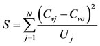 (3)
(3)
In Equation (3), N is the number of sites in the region,  is the coefficient of variation at site j and
  and Uj, are given by Equations (4) and (5)
 (4)
(4)
 (5)
(5)
In Equation (5), nj is the record length at site j and V is the regional variance defined in Equation (6).
 (6)
(6)
In Equation (6), vj is given by
 (7)
(7)
 in Equation (7) is the Cv computed from a sample of size (nj – 1) with the kth observation removed. The statistic S in Equation (4) has the form of a
  statistic. S is expected to be
  distributed with (N – 1) degrees of freedom. If the value of S exceeds the critical value of
  (N – 1) at a particular significance level, then the hypothesis that the region is homogeneous is rejected and the region is regarded as heterogeneous. However, this test is likely to be effective only for large regions having large record lengths. Further developments using distribution-based tests are given by [17] and [18].
The results of the Wiltshire Chi-square statistic was found to be 4.81, which indicates (with a p-value = 0.778) that the eight rainfall stations used could be treated as one region.
Furthermore, the coefficient of skewness and kurtosis are plotted for the stations used in the analysis on the Moment ratio diagrams. For a given distribution, conventional moments can be expressed as functions of the parameters of distributions. It follows that the higher order moments can be expressed as functions of lower order moments. For two-parameter distributions, the moment μ3 can be expressed as a unique function of μ2. For example, the coefficient of skewness (Cs)  can be expressed as a unique function of
 . Similarly,
  of a three-parameter distribution can be expressed as a unique function of Cs. The Cs – Ck moment ratio relationship for some popular three parameter distributions are plotted in what is called the moment ratio diagrams. Cs and Ck moment ratio for the eight stations are also plotted on the same diagram (Figure 2). It shows that both the Generalized Pareto and the Pearson Type III distributions present adequate fits for the eight stations. The Pearson Type III was chosen since it is more known in rainfall frequency analysis. Furthermore, a comparison between the 100-year rainfall value using the Pareto distribution and the Pearson Type III distribution shows a difference of less than 5% in the value, which is negligible for this relatively high return period.
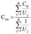
4.2. Index Flood Method for Regionalization
Many types of regionalization procedures are available [13] and [19]. One of the simplest procedures, which has been used for a long time, is the index flood method [20]. The key assumption in the index flood method is that the distribution of the variable of interest at different sites in a region is the same except for a scale or index flood parameter, which reflects rainfall and runoff characteristics of each region. The index flood parameter may be the mean of the maximum annual rainfall, although any location parameter of the frequency distribution may be used [21]. In this case, regional quantile estimates  at a given site for a given return period T can be obtained as in Equation (8), where
  is the quantile estimate from the regional distribution for the given return period, and
  is the mean of the maximum annual rainfall at the site.
 (8)
(8)
The regional distribution parameters are obtained by using the regional weighted average of dimensionless moments obtained by using the dimensionless rescaled data . The joint use of at-site and regional data is advisable, provided that a reasonably homogeneous region can be identified. The data at a site may be used when the record at a station is exceptionally long, or when regional data are not available, or when this site departs somehow from the regional trend.
5. Regionalization Results and Discussion
The fitting of the Pearson Type III distribution to all data using both at site information as well as regional information is shown by Figure 3. It shows that only for three stations (Maquela de Zombo, Noqui and Quinzau) the at-site curve fits the observed data better. This is shown by the closer fit of the at-site blue curve compared to the regional red curve (Figure 3). However, for Noqui station, the 300 mm rainfall value in one day is departing from the global pattern of daily rainfall. Thus, the re-
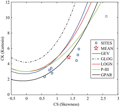
Figure 2. Moment diagrams showing the Eight (8) Stations used in the analysis.
gional estimate, although lower, seems a more reasonable value. Table 9 shows the regional and at-site Pearson type III distribution fittings for 5-, 10-, 25-, 50-, 100-, and 200-year return periods. The values in bold characters are the ones adopted for further analysis. A closer look at the bold values show that the 100-year estimates tend to group geographically in four regions as follows: Landana–Noqui, M Banza Congo, Sazaire (Soyo)–Ambriz–Quinzau, and Maquela de Zombo–Cuimba. This zoning–shown in Figure 1–is undertaken to add more robustness to the values adopted for design.
In the coastal region, The Landana–Noqui axis exhibits the highest rainfall with an average 100-year estimate of 267 mm. The Sazaire (Soyo)–Ambriz axis comes last, with low estimate at Ambriz and relatively higher at Quinzau and average at Sazaire (Soyo).
In the mountainous region, M Banza Congo location reveals higher rainfall than Cuimba and Maquela de Zombo stations. This could be explained by the digital elevation model which reveals that the elevations of Cuimba, Maquela de Zombo and M Banza Congo are 532, 877 and 1000 m, respectively. Furthermore, the Maquela de Zombo station is higher than Cuimba; however it is in the shade of the mountain while Cuimba is in the bottom of the mountain facing the prevailing winds. This might elucidate the reason why Cuimba and Maquela de Zombo experience similar extreme events although there is a difference of elevation between them. Based on the above M Banza Congo is considered in a separate region while as Maquela de Zombo and Cuimba are considered similar and nearly equal to the Sazaire (Soyo)–Quinzau axis. As such, all catchments dischargeing to the ocean in the stretch between Sazaire (Soyo)
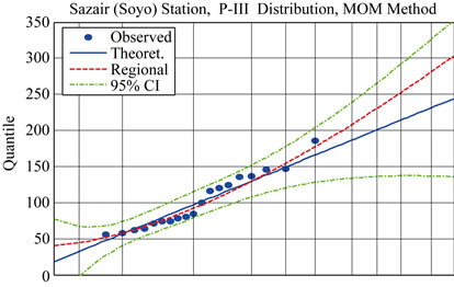

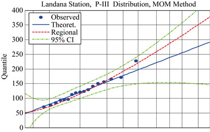


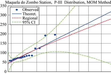

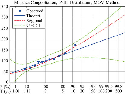
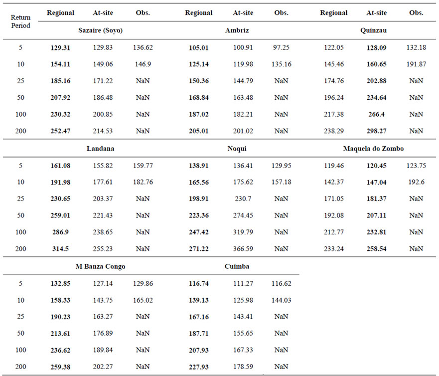
Table 9. Regional and at-site Pearson type III distribution fittings.

Table 10. Adopted daily rainfall values for each zone.

Table 11. Ratios between 24-Hr duration and other storm duration inten-sities.
 (a)
(a)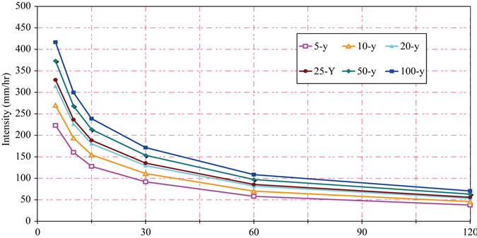 (b)
(b) (c)
(c)
Figure 4. Intensity duration frequency curves for. (a) Landana-Cabinda-Noqui; (b) M Banza Congo; (c) Sazaire (Soyo)- Ambriz-Quinzau and Maquela de Zombo-Cuimba.
and Ambriz are considered to follow the same rainfall pattern because of the similarity between the coastal zone (represented by Sazaire–Ambriz axis) and the mountainous region (represented by Maquela de Zombo– Cuimba zone). The high values depicted in M Banza Congo are only representative of the very high mountain where M Banza Congo is. To calculate the adopted values of daily rainfall at different return periods, a weighted average of the rainfall estimates of Table 9 (based on the length of rainfall record at each location) are calculated for each region. The adopted values are shown in Table 10.
6. Intensity Duration Frequency Curves Development
A theoretical ratio of 1.13 to 1.14 is adopted between daily and 24-hr rainfall values [22]. In the absence of short duration records or any similar information, ratios that could be assumed between intensities of the 24-hr and those of the 12-, 6-, 3-, 2-, 1-Hr, 30-, 15-, and 5-min ratios (refer to Table 11) were first proposed from durations of 2-hr to 5-min by Bell [5] based on studies in the USA, and extended by the Soil Conservation Service of the USA through their SCS type II dimensionless rainfall curve [6]. Using The TRMM data from 3 hours and to 24 hours, we were able to confirm Bell/SCS type II ratios from 3 hours to 24 hours. It is well known that durations from 2 hours to 5 minutes are fairly constant in different climates because of the similarity of convective storms patterns ([5], [23] and references therein).
Based on Tables 10 and 11 and the 24-hour rainfall depths at different return periods, the intensity-duration rainfall values are calculated. IDF curves for return periods of 100-, 50-, 25-, 20-, 10-, and 5-year are shown for the 4 above mentioned zones (Figure 4).
7. Conclusions
This research presents a methodology to overcome the lack of ground station rainfall data by the joint use of the available ground data with TRMM satellite data to develop Intensity Duration Frequency (IDF) curves. Homogeneity of the means and variances are first checked for both types of data. The study zone is verified as being a homogeneous region with respect to frequency analysis using the Wiltshire test. An Index Flood procedure is adopted to generate the theoretical regional distribution equation and the rainfall values at different return periods are calculated for all locations of interest. Regional coherence is identified and used to derive robust rainfall estimates. TRMM data from 3 hours to 24 hours are found consistent with Bell/SCS type II ratios and the Bell/SCS type II are used to develop ratios between 24-hr rainfall depth and shorter duration depths. The regional patterns along with the developed ratios are used to develop regional IDF curves.
8. REFERENCES
- E. Habib, A. Henschke and R. F. Adler, “Evaluation of TMPA Satellite-Based Research and Real-Time Rainfall Estimates during Six Tropical-Related Heavy Rainfall Events over Louisiana, USA,” Atmospheric Research, Vol. 94, No. 3, November 2009, pp. 373-388. doi:10.1016/j.atmosres.2009.06.015
- M. Li and Q. Shao, “An Improved Statistical Approach to Merge Satellite Rainfall Estimates and Raingauge Data,” Journal of Hydrology, Vol. 385, No. 1-4, May 2010, pp. 51-64. doi:10.1016/j.jhydrol.2010.01.023
- M. Almazroui, “Calibration of TRMM Rainfall Climatology over Saudi Arabia during 1998-2009,” Atmospheric Research, Vol. 99, No. 3-4, March 2011, pp. 400-414.
- L. Li, Y. Hong, J. Wang, R. F. Adler, F. S. Policelli, S. Habib, D. Irwn, T. Korme and L. Okello, “Evaluation of the Real-Time TRMM-Based Multi-Satellite Precipitation Analysis for an Operational Flood Prediction System in Nzoia Basin, Lake Victoria, Africa,” Natural Hazards, Vol. 50, No. 1, 2009, pp. 109-123. doi:10.1007/s11069-008-9324-5
- F. C. Bell, “Generalized Rainfall-Duration-Frequency Relationship,” Journal of Hydraulic Division, Vol. 95, No. HY1, 1969, pp. 311-327.
- Soil Conservation Service, “Urban Hydrology for Small Watersheds, Technical Release 55,” United States Department of Agriculture, 1986.
- W. J. Conover, “Practical Nonparametric Statistics,” 3rd Edition, John Wiley, Hoboken, 1980.
- H. B. Mann and D. R. Whitney, “On a Test of Whether One of Two Random Variables is Stochastically Larger than the Other,” Annals of Mathematical Statistics, Vol. 18, No. 1, March 1947, pp. 50-60. doi:10.1214/aoms/1177730491
- F. Wilcoxon, “Individual Comparisons by Ranking Methods,” Biometrics, Vol. 1, No. 6, December 1945, pp. 80- 83. doi:10.2307/3001968
- L. E. Moses, “A Two-Sample Test,” Psychometrika, Vol. 17, No. 3, 1952, pp. 239-247. doi:10.1007/BF02288755
- M. A. Stephens, “EDF Statistics for Goodness of Fit and Some Comparisons,” Journal of the American Statistical Association, Vol. 69, No. 347, September 1974, pp. 730- 737. doi:10.2307/2286009
- H. Levene, “Contributions to Probability and Statistics: Essays in Honor of Harold Hotelling,” Stanford University Press, Palo Alto, 1960, pp. 278-292.
- C. Cunnane, “Statistical Distributions for Flood Frequency Analysis,” Word Meteorological Organization Operational Hydrology Report, No. 33, Geneva, 1989.
- National Research Council, “Committee on Techniques for Estimating Probabilities of Extreme Floods, Estimating Probabilities of Extreme Floods, Methods and Recommended Research”, National Academy Press, Washington D.C., 1988.
- J. R. Stedinger, R. M. Vogel and E. Foufoula-Georgiou, “Frequency Analysis of Extreme Events,” In: D. R. Maidment, Ed., Handbook of Hydrology, McGraw-Hill, New York, 1993.
- A. R. Rao and K. H. Hamed, “Flood Frequency Analysis,” CRC Press, Boca Raton, 2000.
- S. E. Wiltshire, “Regional Flood Frequency Analysis I: Homogeneity Statistics,” Hydrological Sciences Journal, Vol. 31, No. 3, 1986, pp. 321-333. doi:10.1080/02626668609491051
- S. E. Wiltshire, “Identification of Homogeneous Regions for Flood Frequency Analysis,” Journal of Hydraulics, Vol. 84, No. 3-4, May 1986, pp. 287-302. doi:10.1016/0022-1694(86)90128-9
- C. Cunnane, “Methods and Merits of Regional Flood Frequency Analysis,” Journal Hydrology, Vol. 100, No. 1-3, July 1988, pp. 269-290. doi:10.1016/0022-1694(88)90188-6
- T. Dalrymple, “Flood Frequency Analysis, Manual of Hydrology, Part 3, Flood-Flow Techniques: U.S. Geological Survey Water-Supply Paper 1543-A,” 1960.
- J. R. M. Hosking, and J. R. Wallis, “Some Statistics Useful in Regional Frequency Analysis, Res. Rep. RC 17096,” IBM Research Division, New York, 1991.
- D. M. Hershfield, “Rainfall Frequency Atlas of the United States for Durations from 30 Minutes to 24 Hours and Return Periods from 1 to 100 Years,” US Weather Bureau Technical Paper 40, Washington DC, 1962.
- A. G. Awadallah and N. S. Younan, “Impact of Design Storm Distributions on Watershed Response in Arid Regions,” 8th International Association of Hydro-logical Sciences (IAHS) Scientific Assembly, 6-12 September 2009, Hyderabad.