ABSTRACT

The Condon locus for a diatomic molecule is the locus, in the $(v\text{'},v")$ plane, of the strongest bands in an electronic band system. The form of the locus depends upon the form of the potential energy function of the electronic states involved. We show how the locus depends on the potential energy function for simple harmonic and anharmonic oscillators, first from a classical point of view, and then from a quantum mechanical point of view. One phenomenon of interest is that, in the case of anharmonic oscillators, the upper branch of the Condon locus traces much stronger bands than the lower branch. Another phenomenon, predicted by quantum mechanics but not by classical mechanics, is the existence of secondary nested Condon loci.

Keywords:

Diatomic Molecules, Franck-Condon Factors, Condon Locus, Vibrational Constants

1. Introduction

The Franck-Condon factors are factors that give the relative strengths of the many bands in an electronic band system of a diatomic molecule. A band is a transition between the vibrational quantum number $v^{\prime }$ of an upper electronic state and the vibrational quantum number $v^{″}$ of a lower electronic state. Thus a band is defined by the number pair $\left(v^{\prime },v^{″}\right)$ . There is no rigorous selection rule governing such transitions between different electronic states. However, not all such transitions are equally strong. If the Franck-Condon factors are displayed in a table with rows of constant $v^{\prime }$ and columns of constant $v^{″}$, the strongest Franck-Condon factors are often seen to lie on a locus (called the Condon locus) which is roughly a parabola whose symmetry axis makes an angle of about 45˚ to the $v^{\prime }$ and $v^{″}$ axes. This angle may be a little more than 45˚, or a little less. The parabola may be quite narrow (small latus rectum) or quite open (large latus rectum).

A qualitative interpretation for the Franck-Condon loci was originally described by Franck [1] , and a quantum mechanical explanation was developed by Condon [2] . Their physical explanation was described with customary clarity by Herzberg [3] . Roughly it is as follows. At any given instant of time, a molecule is likely to be at its condition of maximum extension or compression, since near these positions in harmonic motion, the speed is slowest. Therefore transitions are most likely to take place from a condition of maximum extension or compression in one electronic state, to a similar condition in the other electronic state. The time taken for an electronic transition is assumed to be very much smaller than the period of vibration of the molecule.

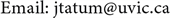
Figure 1 represents the potential energy curves of two electronic states and their quantized total energy levels. It will be seen that a vertical line can easily be drawn from $v^{\prime }=1$ in the upper state to $v^{″}=3$ in the lower state. Thus the $\left(1,3\right)$ band is likely to be strong. Likewise the (2, 0) band is also likely to be strong.

In this paper, we examine the form of the Condon locus at four levels of sophistication:

1) Simple harmonic oscillations, classical treatment.

2) Anharmonic oscillations, classical treatment.

3) Simple harmonic oscillations, wave mechanical treatment.

4) Anharmonic oscillations, wave mechanical treatment.

In addition to the accounts by Condon and Herzberg cited above, one of the most illuminating papers on this topic of which I am aware is that of Nicholls [4] , and there will be some inevitable overlap between that paper and this. However, I have not seen it treated systematically and quantitatively with quite the approach that I am adopting here. Nicholls described the phenomenon of nested Condon loci, which are not predicted classically but which are a result of the wave-mechanical nature of the molecular system.

2. Simple Harmonic Oscillations, Classical Treatment

In the simple harmonic treatment, the potential energy V as a function of internuclear separation r is given by an equation of the form

$V=V_e+\frac{1}{2}k{\left(r-r_e\right)}^2.$ (1)

It is customary in spectroscopic practice to express energies as “term values” T, which are the energies divided by hc, so that the term values are then dimensionally similar (L⁻¹) to wavenumbers. Thus Equation (1) would customarily be written as

$T=T_e+\frac{k}{2hc}{\left(r-r_e\right)}^2.$ (2)

Here $T_e$ is the electronic contribution to the potential energy. The second term on the right hand side is the elastic contribution (of the vibrating molecule) to the potential energy, r is the internuclear distance, and r_e is its equilibrium value. The symbol k is the force constant, related to the molecular vibrational constant ω_e by

$k=4{\text{π}}^{2}m{c}^2{\omega }_e^2$ (3)

where m is the “reduced mass” $\frac{m_1{m}_2}{m_1+m_2}$ of the molecule.

Mathematically the problem is to draw a horizontal line to intersect the upper curve of Figure 1; then drop vertical lines from the two points of intersection; and find the two places where these vertical lines intersect the lower curve. This will result in a relation for the strongest Franck-Condon factors in the form of an equation relating the term values $T^{\prime }$ in the upper electronic state to the term values $T^{″}$ in the lower electronic state.

This relation can then be transferred to the $\left(v^{\prime },v^{″}\right)$ plane via the relations

$T^{″}={T^{″}}_e+\left(v^{″}+\frac{1}{2}\right){{\omega }^{″}}_e$ and $T^{\prime }={T^{\prime }}_e+\left(v^{\prime }+\frac{1}{2}\right){{\omega }^{\prime }}_e$ (4)

The derivation and other details of the analysis are given in Hefferlin et al. [5] and are not repeated here. Suffice it to say that the Condon locus in the $\left(v^{\prime },v^{″}\right)$ plane is a parabola whose equation in a form that is convenient to compute can be written in the form

${\Omega }^{″}\left(v^{″}+\frac{1}{2}\right)={\left(\Delta \pm \sqrt{{\Omega }^{\prime }\left(v^{\prime }+\frac{1}{2}\right)}\right)}^2.$ (5)

In this equation I make use of a quantity

$L=\frac{\hslash }{\text{π}mc}$ (6)

having the dimensions of a length. This is merely to avoid having to repeat $\hslash /\left(\text{π}mc\right)$ in subsequent equations. If m is expressed in amu, L has the numerical value $\frac{6.743052\times {10}^{-17}}{m}$ metres. Then

${\Omega }^{″}=\frac{1}{L{{\omega }^{″}}_e},{\Omega }^{\prime }=\frac{1}{L{{\omega }^{\prime }}_e},\Delta =\frac{{r^{″}}_e-{r^{\prime }}_e}{L}.$ (7)

The properties of the Condon parabola can be traced using any good text on the conic sections (I used my trusty Loney [6] ). The axis of the parabola makes an angle θ with the $v^{″}$ axis given by

$\tan \theta =\frac{{\omega }^{\prime }}{{\omega }^{″}}$ (8)

and the length of the latus rectum is

$2l=\frac{4{\left({r^{″}}_e-{r^{\prime }}_e\right)}^2{{\omega }^{″}}_e^2{{\omega }^{\prime }}_e^2}{L{\left({{\omega }^{″}}_e^2+{{\omega }^{\prime }}_e^2\right)}^{3/2}}.$ (9)

The parabola is tangent to the lines $v^{\prime }=\frac{1}{2}$ and $v^{″}=\frac{1}{2}$ .

If the equilibrium internuclear separations in the two electronic states are equal, the parabola degenerates into a straight line. A wide Condon parabola indicates that the internuclear separations in the two electronic states are rather different. I show, in Table 1 and Figure 2, two examples, in one of which, CN $B^2{\Sigma }^{+}-X^2{\Sigma }^{+}$, the internuclear distances in the two states are not very different and the Condon parabola is consequently rather narrow; and in the other, AlO $A^2{\Pi }_r-X^2{\Sigma }^{+}$, the internuclear distances are rather different, and the Condon parabola is broad.

In the classical model, a simple harmonic oscillator is most likely to be found, at some instant of time, at one of the extrema of its motion. The probability that its distance ξ from its equilibrium position will be between ξ and ξ + dξ is proportional to the reciprocal of its speed (by which I mean $\text{d}r/\text{d}t$ rather than the speed of one of the atoms), which I shall call its “slowness”, s. The time spent in traversing a distance dξ is sdξ. Indeed the probability that the position of the system will, at some instant of time, be in the interval dξ is $2s\text{d}\xi /P=\omega s\text{d}\xi /\text{π}$ . Here P is the period of the motion, and ω (not to be confused with the vibrational constant ω_e) is 2π/P. The factor 2 on the left hand side of the equation arises because the displacement from equilibrium passes through ξ twice per period. And, since the speed in simple harmonic motion of amplitude a is $\omega \sqrt{a^2-{\xi }^2}$, the probability $\text{d}\Phi$, at some instant, that the displacement will be between ξ and ξ + dξ is

$\text{d}\Phi =\frac{2\text{d}\xi }{\text{π}\sqrt{a^2-{\xi }^2}}.$ (10)

The coefficient of dξ, which I may call the probability density, is shown graphically in Figure 3 for a = 1. The integral between $\xi =0$ and $\xi =a$ is unity, as befits a probability. The function goes to infinity at $\xi =\pm a$, but of course $\text{d}\Phi$ is everywhere finite (zero) as $\text{d}\xi \to 0$ .

3. Anharmonic Oscillations, Classical Treatment

The vibration of a real molecule will not be simple harmonic, and the curve representing its potential energy as a function of internuclear distance will not be a parabola. For small internuclear distances, when the molecule is compressed, there will be a strong Coulomb repulsion between the nuclei, so the potential energy curve there is steep and negative. For large internuclear distances, the molecule will tend to dissociate, so the potential energy curve asymptotically approaches a dissociation limit. Qualitatively the potential energy function would be expected to look somewhat similar to one of the curves shown in Figure 4. (The small difference between these curves will be described later, following Equation (15)).

The same principles apply in forming the Condon locus as in the simple harmonic case, except that the Condon locus will no longer be a parabola. Transitions are most likely to take place near the stationary points (greatest extension or compression) of the vibration as before. However, if one were to imagine a particle sliding without friction to and fro in one of the potential wells of Figure 4, it is easy to conclude that the particle will spend more time at large r than at

small r. That means that transitions are more likely to occur when the molecule is at greatest extension than at greatest compression. This leads to the conclusion, by qualitative argument alone and without any numerical calculation, that the upper branch of the Condon locus traces much stronger bands than the lower branch. We shall see later that the wavemechanical treatment leads to the same conclusion.

Various attempts can be made to devise empirical equations that mimic the expected qualitative potential curve. Two of them are the Morse potential [7] and the Lennard-Jones potential [8] .

The Morse potential is

$V=D_e{\left[1-{\text{e}}^{-\left(r-r_e\right)/a}\right]}^2.$ (11)

V = potential energy as a function of the internuclear distance r. r_e = equilibrium internuclear distance. D_e = dissociation energy. The parameter a has the dimensions of length. What little geometric meaning we can give to a is such that when $r-r_e=a$,

$V={\left(1-{\text{e}}^{-1}\right)}^2{D}_e=0.399576D_e\approx 0.4D_e.$ (12)

That is to say the extension of the molecule from its equilibrium separation is a when the potential energy is about 40 percent (i.e. 0.399576) of the dissociation energy. Alternatively, when the potential energy is half of the dissociation energy, the extension or compression is

$r-r_e=\ln \left(2\pm \sqrt{2}\right)=1.2279aor-0.5348a.$ (13)

There is another formal solution, namely when $r_e-r=a$,

$V={\left(1-e\right)}^2{D}_e=2.952D_e,$ (14)

but this is not a physically interesting solution, because if $V>D_e$, the molecule is unstable. If the molecule is compressed by an amount $r_e-r=a$, it will bounce back and dissociate.

The Lennard-Jones potential is

$V=D_e\left[1+{\left(\frac{r_e}{r}\right)}^m-2{\left(\frac{r_e}{r}\right)}^n\right].$ (15)

In Figure 4, the dashed line is a Lennard-Jones potential with m = 12 and n = 6, while the continuous line is a Morse potential with a = 0.1772. Some slightly tedious algebra will show that the Morse and Lennard-Jones potentials (with m = 12 and n = 6) will have the same full widths at half minimum (FWHm) for

$a=\frac{{\left(2+\sqrt{2}\right)}^{1/6}-{\left(2-\sqrt{2}\right)}^{1/6}}{\ln \left(3+\sqrt{8}\right)}=0.177212908,$ (16)

which is the reason why I chose that value for the Morse parameter in preparing Figure 4.

Although the two curves look somewhat similar, only the Lennard-Jones function has the physically desirable characteristic of going to infinity as $r\to 0$ . However, the Morse function is very steep for small r, and, in the example of Figure 4, it reaches the respectable value of $7.9\times {10}^4$ at r = 0, so that the function does not give a wholly unreasonable representation of a real potential function. Another attractive feature of the Morse function is that, when it is inserted into the Schrödinger equation, the eigenfunctions can be written explicitly in terms of algebraic functions (Laguerre polynomials), and, especially, the eigenvalues (vibrational energy levels) are given as

$T=T_e+G\left(v\right)=T_e+{\omega }_e\left(v+\frac{1}{2}\right)-{\omega }_e{x}_e{\left(v+\frac{1}{2}\right)}^2,$ (17)

with no higher powers of $\left(v+\frac{1}{2}\right)$ . For these reasons I use the Morse function

in the present analysis of anharmonicity. (In Equation (17), T is the energy divided by hc. That is to say, it is the term value (in m⁻¹) of the level.)

Further comparisons between these two potential functions can be found in Lim [9] .

Let us introduce the dimensionless variables

$\xi =\left(r-r_e\right)/a.$ (18)

and

$U=V/D_e$ (19)

Then the Morse function is

$U={\left(1-{\text{e}}^{-\xi }\right)}^2.$ (20)

The Taylor expansion of this to ξ² is just $U={\xi }^2$ . Thus, to order ξ², the Morse potential is the same as the simple harmonic oscillator potential for which

$V=\frac{1}{2}k{\left(r-r_e\right)}^2$

where k is the force constant, and hence

$a=\sqrt{2D_e/k},k=2D_e/a^2.$ (21)

The fundamental frequency is

${\nu }_0\text{}\text{}\text{}=\frac{1}{\text{2π}}\sqrt{\frac{k}{m}}=\frac{1}{2\text{π}a}\sqrt{\frac{2D_e}{m}},$ (22)

and the following relations are also of interest:

${\omega }_e=\frac{{\nu }_0}{c},{\omega }_e{x}_e=\frac{h{\nu }_0^2}{4D_{e}c}.$ (23)

For large a (small force constant), the graph of the potential energy versus r − r_e has a wide and shallow minimum. For small a, the graph of the potential energy versus r − r_e has a sharp and steep minimum. Figure 5 shows a Morse curve with its energy levels.

In Figure 5, ξ is $r-r_e$ in units of a, and, for reference, the energies of the v th levels and the limits of the motion are given in Table 2.

The Condon locus resulting from transitions between two electronic states whose potential energies are given by Morse functions can be found by the same

procedure as for simple harmonic functions, as described following Equation (3) in Section 2. Because of the transcendental nature of the equations, it is not possible to arrive at a simple, explicit equation for the Condon locus (which is no longer a parabola). It is straightforward, in any particular case, to carry out the procedure numerically by computer. Transformation from the $\left(T^{\prime },T^{″}\right)$ plane to the $\left(v^{\prime },v^{″}\right)$ plane is performed by inversion of Equation (17). The electronic contributions to the energies of the two states do not come into the Condon locus in the $\left(v^{\prime },v^{″}\right)$ plane, and can both conveniently be taken to be zero.

I have done the calculations for several cases below, in Figure 6, where we can see how the nature of the Condon locus varies with the molecular constants of the two states. Except for the anharmonicity constants ${{\omega }^{\prime }}_e{x^{\prime }}_e$ and ${{\omega }^{″}}_e{x^{″}}_e$, I have used the molecular constants for the CN $B^2{\Sigma }^{+}-X^2{\Sigma }^{+}$ tabulated in Section 2, Table 1. For illustrative purposes I have added various purely fictional values of ${{\omega }^{\prime }}_e{x^{\prime }}_e$ and ${{\omega }^{″}}_e{x^{″}}_e$, shown in Table 3 in order to see their effect on the Condon locus. The dashed curves show the Condon parabola in the simple harmonic approximation, in which ${{\omega }^{\prime }}_e{x^{\prime }}_e$ and ${{\omega }^{″}}_e{x^{″}}_e$ are both zero. The full lines are the Condon loci when anharmonicity is added. I have drawn the upper arm of the Condon locus in the anharmonic case with a thicker line than the lower arm, to reflect the fact that, as explained in the second paragraph of this Section, the upper arm delineates stronger Franck-Condon factors than the lower arm. The values chosen for the anharmonic constants are indicated in Table 3. Since a picture is worth a thousand words, I leave it to the reader to discern the trends that arise from various choices of the anharmonicity constants.

As in the simple harmonic case, the probability that the position of the system will, at some instant of time, be in the interval dξ is $2s\text{d}\xi /P$, where s is the slowness and P is the period, though determining this quantity is slightly less easy that in the simple harmonic case. For illustrative purposes I shall consider a Morse potential of the form given by Equation (11) and I shall determine expressions for the period P of the motion and the slowness s as a function of ξ.

The period P of the motion, in units of $a\sqrt{m/D_e}$ (a-Morse parameter, m = reduced mass of the molecule, D_e = dissociation energy), is

$P=\sqrt{2}\left[{\displaystyle {\int }_{{\xi }_{\text{left}}}^0\frac{\text{d}\xi }{\sqrt{E_v-{\left(1-{\text{e}}^{-\xi }\right)}^2}}}+{\displaystyle {\int }_0^{{\xi }_{right}}\frac{\text{d}\xi }{\sqrt{E_v-{\left(1-{\text{e}}^{-\xi }\right)}^2}}}\right],$ (24)

where E_v is the total energy in the vth vibrational level. The first integral pertains to the time when the molecule is compressed; the second integral pertains to the time when the molecule is extended. The integration results in

$P=\sqrt{\frac{8}{1-E_v}}\left[{\tan }^{-1}\left(\frac{1-\sqrt{E_v}}{\sqrt{1-E_v}}\right)+{\tan }^{-1}\left(\frac{1+\sqrt{E_v}}{\sqrt{1-E_v}}\right)\right].$ (25)

Table 4 shows, for the first eight vibrational levels, the time P₁, in units of $a\sqrt{m/D_e}$, during which the molecule is compressed; the time P₂ during which it is extended; the total period P; and the ratio P₂/P₁. It will be seen that this ratio increases with vibrational quantum number. This means that our prediction that the upper arm of the Condon locus delineates stronger Franck-Condon factors than the lower arm is more pronounced at larger quantum numbers, and less pronounced at lower quantum numbers.

The speed (i.e. $\text{d}r/\text{d}t$ ) in units of $\sqrt{D_e/m}$ as a function of internuclear distance is given by (nonrelativistic) energy considerations to be

$\frac{\text{d}r}{\text{d}t}=\sqrt{2\left[E_v-{\left(1-{\text{e}}^{-\xi }\right)}^2\right]},$ (26)

where $\xi =\left(r-r_e\right)/a$, and the slowness s is the reciprocal of this. The probability density 2s/P is shown in Figure 7 as a function of ξ for the ν = 7 level. The area under the curve is unity. Table 4 and Figure 7 show that the molecule spends more time in extension $\left(\xi >1\right)$ than in compression $\left(\xi <1\right)$, with the consequence that the upper arm of the Condon locus is stronger than the lower arm; and that for large v the molecule spends much more time in extension than in compression, with the consequence that in practice the lower arm of the Condon locus is likely to be observed only for low ν.

4. Simple Harmonic Oscillations, Wave Mechanical Treatment

In the wave mechanical model, the probability density, denoted by the symbol ψ², is a wavefunction with several nodes (zeroes) and antinodes (maxima), and which extends slightly beyond the classical limits of the motion. At a given instant of time, the extension of a molecule from its equilibrium position is most likely to be at one of the maxima of ψ². And, since there are several maxima, this gives rise to the possibility that there will be, in the $\left(v^{\prime },v^{″}\right)$ plane, several nested Condon loci delineating strong Franck-Condon factors. Examples of such nested Frank-Condon factors will be found in Nicholls [4] .

For simple harmonic potentials the wavefunctions are given in many standard texts, such as that of Eyring, Walter and Kimbal [10] . Normalized to unit area they are

${\psi }^2=\frac{1}{2^{v}v!\sqrt{\text{π}}}\frac{H_v^2\left(\xi \right){\text{e}}^{-{\xi }^2}}{l}$ (27)

where

$l=\sqrt{\frac{\hslash }{\sqrt{mk}}}$ (28)

and the $H_v$ are the Hermite polynomials. The constant l has dimensions of length. (Recall that ${\psi }^2\text{d}r$ must be dimensionless, which verifies that Equation (27) balances dimensionally.) Samples of these, for $v=0,5,10$ are shown in Figures 8-10, where the vertical lines are the classical limits of the motion.

Several features are worthy of comment. For large v the locus of the maxima closely follow the probability density for the classical case illustrated in Figure 3, and this is often cited as an example of the Bohr correspondence principle. The molecule, at some instant, is most likely to be found near (but not exactly at) the extrema of the motion. The subsidiary maxima are rather lower than the main maxima, which means that the Franck-Condon factors that they delineate will not be as strong as those delineated by the principal maxima. For intermediate ν these characteristic are not at all as pronounced, while for ν = 0 (no vibration)

the most likely condition of the molecule is not at an extremum of the potential well, but it will most likely be at its equilibrium position, which will surprise no one.

It is evident that, in order to calculate the Condon loci, we need to know the positions of the maxima of these wavefunctions. These are given in Table 5.

By way of example of the principles involved, I draw in Figure 11 two simple harmonic potential energy curves for a fictitious molecule. I am taking the potential energy of the two electronic states involved to be

$V=V_e+\frac{1}{2}k{\left(r-r_e\right)}^2,$ (29)

where for the lower state,

$V_e=0,\frac{k}{2hc}=2.447\times {10}^{25}{m}^{-3},r_e=3.9\times {10}^{-10}m$ (30)

and for the upper state,

$\frac{V_e}{hc}=2\times {10}^5{m}^{-1},\frac{k}{2hc}=1.625\times {10}^{25}{m}^{-3},r_e=4.0\times {10}^{-10}m.$ (31)

In Figure 11 I have drawn the first eleven vibrational energy levels in each electronic state, and I have indicated by dots the positions of the maxima of the squares of the wavefunctions. The heights of these maxima can be found from Table 5 and from Figures 8-10. At a given instant of time the most probable condition of the molecule is not that of greatest extension or compression, but at a separation corresponding to the position of one of the dots. A likely transition (i.e. a large Franck-Condon factor) is one for which a dot on a level in the lower state is vertically beneath a dot on a level in the upper state (on the supposition that the time taken for an electronic transition is much shorter than the vibrational period of the molecule).

I have also indicated, by dashed curves in the figure the approximate loci of the largest and the second largest maxima. These loci are not exact parabolas, although in the drawing I have indicated the “best” parabolas (quadratic least squares regressions of r upon V) through the dots.

These loci can now be used to calculate Condon loci in the $\left(v^{\prime },v^{″}\right)$ plane, which are shown in Figure 12. The full curve is the Condon locus for simple harmonic oscillations, classical treatment. The dashed curves are the loci of the most prominent bands according to the wavemechanical calculations. In addition to large Franck-Condon factors delineated along the Condon loci, there may also be a few strong bands randomly distributed. For example, reference to Figure 11 shows that there will be a strong band joining a secondary maximum at $v^{\prime }=8$ to a principal maximum at $v^{″}=7$ .

5. Anharmonic Oscillations, Wave Mechanical Treatment

The Morse potential is given by Equation (11). When this is inserted into the Schrödinger equation, it is well known that the eigenvalues (energy levels) can be written as a series in $v+\frac{1}{2}$ containing no powers higher than the second. The energy levels are given by

$E_v=h{\nu }_0\left[\left(v+\frac{1}{2}\right)-\frac{h{\nu }_0}{4D_e}{\left(v+\frac{1}{2}\right)}^2\right]$ (32)

In spectroscopic practice, this is usually written as vibrational term values $G\left(v\right)$ (energy divided by hc) and the vibrational and anharmonicity constants ${\omega }_e$ and ${\omega }_e{x}_e$ :

$G\left(v\right)={\omega }_e\left(v+\frac{1}{2}\right)-{\omega }_e{x}_e{\left(v+\frac{1}{2}\right)}^2$ (33)

from which we see that

${\omega }_e=\frac{{\nu }_0}{c}$ (34)

and

${\omega }_e{x}_e=\frac{h{\nu }_0^2}{4D_{e}c}$ (35)

Another way of writing equations (32) or (33) is

$\frac{E_v}{D_e}=b\left[\left(v+\frac{1}{2}\right)-\frac{1}{4}{\left(v+\frac{1}{2}\right)}^2\right]$ (36)

where b (dimensionless) is

$b=\frac{h{\nu }_0}{D_e}$ (37)

Figure 5 was drawn with an arbitrary value of $b=\frac{1}{4}$ .

I also introduce, for convenience, some more quantities as follows:

$\hat{E}=\frac{h^2}{2m{a}^2}=\frac{{\text{π}}^2{c}^2{\hslash }^2{\omega }_e^2}{D_e}=\frac{c^2{h}^2{\omega }_e^2}{4D_e}=\frac{1}{4}{b}^2{D}_e.$ (38)

$\beta =\frac{1}{b}=\frac{D_e}{h{\nu }_0}$ (39)

$z=4\beta {\text{e}}^{-\xi }$ (40)

$P=v!{\left[\frac{4\beta -v-1}{\Gamma \left(v+1\right)\Gamma \left(4\beta -v\right)}\right]}^{1/2}$ (41)

$Q=z^{2\beta -\left(v+\frac{1}{2}\right)}{\text{e}}^{-z/2}$ (42)

$R=L_v^{4\beta -2v-1}\left(z\right)$ (42)

where the L are the Laguerre polynomials, generated by

$L_v^n\left(z\right)=\frac{z^{-n}{\text{e}}^z}{v!}\frac{{\text{d}}^v}{\text{d}{z}^v}\left(z^{n+v}{\text{e}}^{-z}\right).$ (43)

Of these quantities, $\hat{E}$ has dimensions of energy, while the others are dimensionless.

The wavefunctions for the Morse potential are then given by

${\psi }_v\left(z\right)=PQR{a}^{-1/2}.$ (44)

The quantity P is the normalization factor chosen to ensure that ${\displaystyle {\int }_0^{\infty }{\psi }^2\text{d}r}=1$ . In this paper I am concerned only with the Condon loci and hence only with the positions and relative heights of the maxima of the wavefunctions. Thus I shall be concerned only with the ξ-dependent part of the wavefunctions, namely the product QR. The Morse function of Figure 5 was drawn with$b=\frac{1}{4},\beta =4$, and I tabulate below, in perhaps a more comprehensible form than Equation (44), the unnormalized wave functions (i.e. the product QR) for the first eight vibrational levels.

${\psi }_0=z^{7.5}{\text{e}}^{-z/2}$ (45)

${\psi }_1=\left(14-z\right)z^{6.5}{\text{e}}^{-z/2}$ (46)

${\psi }_2=\frac{1}{2}\left(156-26z+z^2\right)z^{5.5}{\text{e}}^{-z/2}$ (47)

${\psi }_3=\frac{1}{6}\left(1320-396z+36z^2-z^3\right)z^{4.5}{\text{e}}^{-z/2}$ (48)

${\psi }_4=\frac{1}{24}\left(7920-3960z+660z^2-44z^3+z^4\right)z^{3.5}{\text{e}}^{-z/2}$ (49)

${\psi }_5=\frac{1}{120}\left(30240-25200z+7200z^2-900z^3+50z^4-z^5\right)z^{2.5}{\text{e}}^{-z/2}$ (50)

$\begin{array}{c}{\psi }_6=\frac{1}{720}(60480-90720z+45360z^2-10080z^3\\ +1080z^4-54z^5+z^6)z^{1.5}{\text{e}}^{-z/2}\end{array}$ (51)

$\begin{array}{c}{\psi }_7=\frac{1}{5040}(40320-141120z+141120z^2-58800z^3\\ +11760z^4-1176z^5+56z^6-z^7)z^{0.5}{\text{e}}^{-z/2}\end{array}$ (52)

By way of example I draw, in Figures 13-15, the squares of the unnormalized wavefunctions ( $Q^2{R}^2$ ) for ν = 0, 4 and 7. The vertical dashed lines indicate the classical limits of the motion.

As in the classical model, we see that, for large v, the molecule spends much more time in extension than in compression, so that the lower arm of the Condon locus is likely to be observed only for very small v. And, as for the simple harmonic case, for large v, the locus of the maxima becomes more and more similar to the classical “slowness” curve of Figure 7, providing another example of the correspondence principle.

The strongest bands in a band system depend immediately on the positions of the maxima of the squares of the wavefunctions. Accordingly I provide, for the first eight vibrational levels, these positions in Table 6, in which the entries in normal font are the values of ξ at which ψ² is a maximum, and boldface entries are the classical limits of the motion.

As with the simple harmonic case of Section 4, I draw as Figure 16, by way of example of the principles involved, two anharmonic potential energy curves for

a fictitious molecule. The potential energy curves are calculated with the (arbitrary but realistic) values given in Table 7.

The dots in Figure 16 indicate the positions of the maxima of the squares of the wavefunctions. These dots give the most probable extension or compression

at any instant of time. The magnitudes of ψ² at each of these position are given in Table 6 and Figures 13-15. The loci of the strongest maxima are shown by dashed curves.

The Condon loci have to be determined numerically by the following procedure. We start with some value of the upper vibrational quantum number $v^{\prime }$ and determine the corresponding term value $T^{\prime }=V^{\prime }/hc$ from Equation (17). We then determine the two values of the internuclear distance corresponding to this term value from the dashed loci in the upper state of Figure 16. Then determine the term values of the lower state corresponding to these internuclear distances from the dashed curves of the lower state. Finally calculate the corresponding values of $v^{″}$ from the converse of Equation (17).

In Figure 17 I show the principal Condon locus as a dashed curve. The full curve shows the “classical” locus for Morse (anharmonic) potential functions-i.e. the locus calculated on the assumption that the most likely internuclear separation at any given instant is that of full compression or full extension, rather than at the maxima of the eigenfunctions.

I have not shown any secondary loci, because the possibilities are almost endless, quantum numbers of the strong and weak bands being almost random. Strong bands occur wherever the internuclear separation corresponding to a maximum in the eigenfunction in the upper state corresponds with a maximum in the lower state at the same internuclear separation. In terms of Figure 16, and expressed more simply, there is a strong band wherever a dot in the upper part of Figure 16 is vertically above a dot in the lower part.

It will be understood from this that small differences in the shapes and positions of the potential curves (i.e. in the equilibrium internuclear distances and the vibrational constants) will result in differences in the positions of the dots

and hence in the designations of the bands that are likely to be strong or weak. It will also be understood that if the two potential curves are quite similar, secondary and tertiary Condon loci will be much more likely. Indeed, it could be advanced that, if a secondary Condon locus is very evident, it is likely that the internuclear separations of the two electronic states are not very different. Unfortunately in that case the entire electronic band system is likely to be weak because of the small difference in electric dipole moments of the two electronic states, and also, as noted in Section 2, the Condon locus is likely to be narrow and the strongest bands are those in which $\Delta v$ is small.

6. Comparison with Observation

The thrust of this paper has been primarily theoretical. However, calculations of the predicted Condon loci, including in the simple harmonic case the latera recta of the Condon parabolas and the inclinations of their axes, have been carried out for 47 electronic band systems and compared with observations. The results for these are given in Hefferlin et al. [5] .

Acknowledgements

I would like to thank Rev. Dr Ray Hefferlin of Southern Adventist University, Tennessee, for his encouragement and for exciting my interest in this problem during his continuing studies of the systematics of molecular spectroscopic constants.

Conflicts of Interest

The authors declare no conflicts of interest regarding the publication of this paper.

Cite this paper

Tatum, J.B. (2018) Theory of the Condon Locus. Journal of Modern Physics, 9, 1735-1760. https://doi.org/10.4236/jmp.2018.99109

References

- 1. Franck, J. (1925) Transactions of the Faraday Society, 21, 536-542. https://doi.org/10.1039/tf9262100536
- 2. Condon, E.U. (1928) Physical Review, 32, 858-872. https://doi.org/10.1103/PhysRev.32.858
- 3. Herzberg, G. (1950) Molecular Spectra and Molecular Structure. I. Spectra of Diatomic Molecules, Van Nostrand, Princeton, 194-204.
- 4. Nicholls, R.W. (1982) Journal of Quantitative Spectroscopy & Radiative Transfer, 28, 481-492. https://doi.org/10.1016/0022-4073(82)90014-0
- 5. Hefferlin, R., Sackett, J. and Tatum, J.B. (2012) Systematics and Prediction in Franck-Condon Factors, in Quantum Systems in Chemistry and Physics. Springer, Dordrecht, 179-191. https://doi.org/10.1007/978-94-007-5297-9_8
- 6. Loney, S.L. (1895) The Elements of Coordinate Geometry. MacMillan, London, 359-363.
- 7. Morse, P.M. (1929) Physical Review, A34, 57-64. https://doi.org/10.1103/PhysRev.34.57
- 8. Lennard-Jones, J.E. and Dent, B.M. (1926) Proceedings of the Royal Society, A112, 230-234. ttps://doi.org/10.1098/rspa.1926.0107
- 9. Lim, T.-C. (2003) Zeitschrift für Naturforschung, 58a, 615-617. https://doi.org/10.1515/zna-2003-1104
- 10. Eyring, H., Walter, J. and Kimball, G.E. (1944) Quantum Chemistry. Wiley, New York, 75-79.