Journal of Modern Physics
Vol.3 No.9(2012), Article ID:22615,16 pages DOI:10.4236/jmp.2012.39118
Quasi Non-Markovian Approach to the Study of Decoherence of a Controlled-Not Quantum Gate in a Chain of Few Nuclear Spins Quantum Computer
Departamento de Física, Universidad de Guadalajara, Guadalajara, Mexico
Email: pablocarloslopez@hotmail.com, gulopez@udgserv.cencar.udg.mx
Received June 20, 2012; revised July 19, 2012; accepted July 27, 2012
Keywords: Decoherence; Chain of Nuclear Spins; Controlled-Not
ABSTRACT
We develop in the weak coupling approximation a quasi-non-Markovian master equation and study the phenomenon of decoherence during the operation of a controlled-not (CNOT) quantum gate in a quantum computer model formed by a linear chain of three nuclear spins system with second neighbor Ising interaction between them. We compare with the behavior of the Markovian counterpart for temperature different from zero (thermalization) and at zero temperature for low and high dissipation rates. At high dissipation there is a very small difference between Markovian and quasi no-Markovian at any temperature which is unlikely to be measured, and at low dissipation there is a difference which is likely to be measured at any temperature.
1. Introduction
A quantum open system is generally characterized by a non unitary evolution of the reduced density matrix associated to the central system and its interaction with the environment. Different types of approaches have been developed to understand the phenomenon of decoherence that arises in the open quantum systems which it is related to the lost of the interference terms of the product of the quantum wave function [1-8], that is, the non diagonal elements of the reduced density matrix go to zero value. Since the complete insulate quantum system is almost impossible to have, decoherence becomes an intrinsic phenomenon related to the quantum principles and maybe related to the “emergent reality” of the classical world [9-13]. Many interests have been created in the phenomenon because of the difficulties it carries to perform quantum computation. Non-Markovian systems or systems where the environment is supposed to keep memory, is a topic in this subject and there is not a unified consensus about the best approach for studying the dynamics of this systems [14-18] which makes nonMarkovian to be a very interesting subject. In the Markovian approach the non-unitary evolution equation is called “master equation” which is a differential equation for the traced over the environmental variables of the full density matrix. In principal, in the non-Markovian approach one will have to obtain an integro-differential equation for the density matrix and to establish the nonMarkovian in it, but, how to measure non-Markovian? It is still uncertain. Every approach needs to be intended to maintain the positiveness and trace equal to one for the reduced density matrix. The best known mathematical formalism which kept these conditions was given by Lindblad [4], who gave an abstract general non unitary evolution equation for the reduced density matrix, so keeping the Lindblad form in the equations is a good indication. We thought in quasi non-Markovian as an approximation to a master equation but with a temporal dependence in some of the coefficients which defines the interaction with the environment which also depends on the Ising interaction between the spins and may lead to a different behavior of the traditional Markovian solutions. In addition, these solutions keep the completely positiveness of the density matrix.
We use the weak coupling approximation for a system consisting of a linear chain of three paramagnetic atoms with nuclear spin one half [19], interacting with a thermal reservoir (not pure) consisting of a bosonic bath [20- 22]. The temporal dependence in some terms, in the weak coupling approximation, is what we have considered as something beyond Markovian which is totally related to this type of system, and more specifically, to the Ising interaction between the nuclear spins.
We study the decoherence of quantum controlled-not (CNOT) gates during operation in a quantum computer model. In this work, we are interested in determine the differences between the quasi-non-Markovian and Markovian behavior of a quantum controlled-not (CNOT) gate during its implementation on this model of quantum computer. In the first part of this work, we describe this model and the Hamiltonian of our quantum system interacting with a thermal reservoir, which consist of modes of an electromagnetic field in a cavity where the quantum system is. In the second part, we perform the weak coupling approximation to obtain a quasi-nonMarkovian master equation. We want to point out that, even when this model has not been built, it has been very useful for theoretical studies about implementation of quantum gates and quantum algorithms [23-25] which can be extrapolated to other solid state quantum computers [26]. Then, the analytical dynamical system of the reduced density matrix elements are obtained, and the results of the numerical simulations are presented. We present mainly the differences between the Markovian and the quasi-non-Markovian behavior on the reduced density matrix elements.
2. Hamiltonian of the System
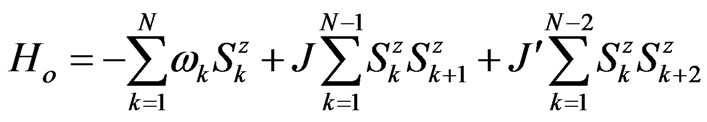
The Hamiltonian that describes the ideal insulated system of a linear chain of N paramagnetic atoms with nuclear spin one half inside a magnetic field
 (1)
(1)
where  and
and  are the amplitude, the angular frequency and the phase of the RF-field, and
  represents the amplitude of the z-component of the magnetic field, is given by [23]
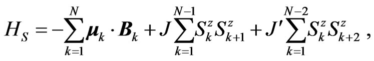 (2)
(2)
where  represent the magnetic moment of the kthnucleus, which it is given in terms of the nuclear spin as
 , with
  being the proton gyromagnetic ratio and
  being the jth-component of the spin operator,
  represents the magnetic field Equation (1) valuated at the location of the kth-nuclear spin
 . The parameters
  and
and  represent the coupling constant at first and second neighbor interaction. The angle between the linear chain and the z-component of the magnetic field is chosen as
  to eliminate the dipole-dipole interaction between the spins.
We can write the Hamiltonian (2) in its diagonal and non diagonal with respect a chosen basis in the z-projection as
 (3)
(3)
where
 (4)
(4)
and
 (5)
(5)
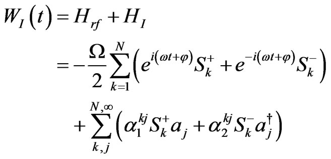
Here we have that:  is the Larmor frequency of the kth-spin,
  is the Rabi frequency, and
  represents the ascend operator (+) or the descend operator (−). The Hamiltonian
  is diagonal in the basis
  with
with  (one for the ground state and zero for the exited state). The action of the spin operators on its respective qubit is given by
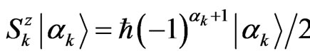 ,
, 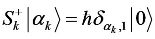 , and
, and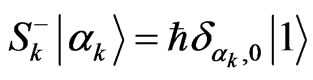 . The eigenvalues of
  in this basis are given by
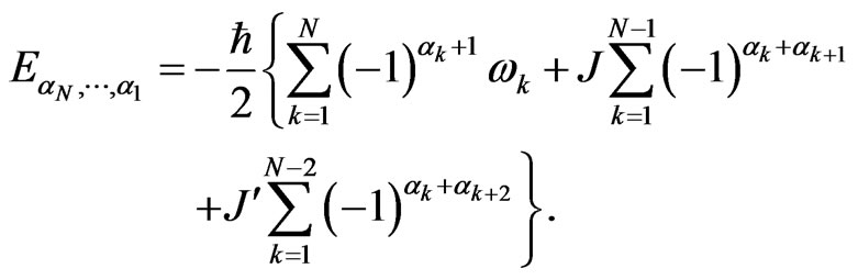 (6)
(6)
The elements of this basis forms a register of N-qubits with a total number of  registers, which is the dimensionality of our Hilbert space. The allowed transition of one state to another one is gotten by choosing the angular frequency of the RF-field,
  , as the associated angular frequency due to the energy difference of these two levels, and by choosing the normalized evolution time
  with the proper time duration (so called RFfield pulse). The set of selected pulses defines the quantum gates or the quantum algorithms, and CNOT quantum gate is the gate we want to study.
Consider now this system to be immerse in a “mixed thermal bath of oscillators” such that the Hamiltonian of the bath is of the form
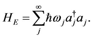 (7)
(7)
The Hamiltonian of the interaction between the central system and the bath will be taken in the form
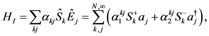 (8)
(8)
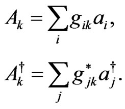
where the operator  is defined as
 ,
,  is the polarization operator,
  , and we have taken into account the Jaymes-Cummings rotating wave approximation for the interaction [27], in order to considerer an excitation-de excitation process of the system trough the coupling with the bath of oscillators with characteristic frequencies near the resonant frequencies of the transitions. The constants
 ,
,  are phenomenological parameters that measures the coupling between the system and the environment and
  are the rising (lowering) operators in jth number of photons in the bath. We can write the total Hamiltonian as
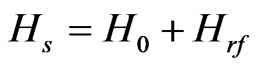
 (9)
(9)
where  and
and  are given by
 (10)
(10)
and
 (11)
(11)
3. The Weak Coupling Approximation
Now, for dealing with the non ideal situation we start with the dynamical equation of the evolution of the density matrix for an initially decoupled state in the system plus the environment
 (12)
(12)
where  is a pure state of the central system and
  is a thermal stationary mixed state of the environment. In the interaction picture the equation of evolution for the reduced system is
 (13)
(13)
where in this interaction picture one has
 (14)
(14)
 (15)
(15)
and
 (16)
(16)
with the operator  being defined as
 (17)
(17)
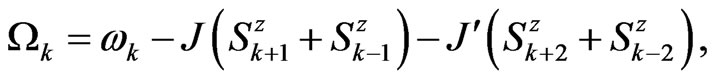
which commutes with the Hamiltonian . The eigenvalues of this operator
 ,
,
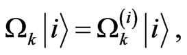 (18)
(18)
are given in the Appendix.
The time integration of the system in the interval  is given as follows
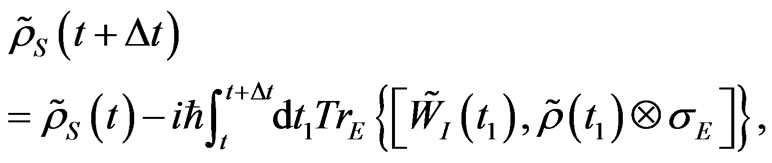 (19)
(19)
Then by doing a successive change of variables and substituting in (19), up to second order terms, using Markov approximation and Equation (12), we obtain
 (20)
(20)
where time locality is shown inside the integration with the term , and we have set
 . One would expect that within this weak coupling approximation, the interaction of the central system with the environment would show a perturbation to the closed system. By substituting the corresponding time dependence form of
  in (20), one can sees that the following relation must be satisfied (notice that
  for all basic state
 )
)
 (21)
(21)
which determine the time path length where there is no interaction with a time dependent external field and no interaction between the spins How smaller this path has to be is not resolved, but definitively not that small compared to the relaxation times of the environment  such that the Markov approximation still being valid. The lost of the separability of the initial system-environment states
  for a smaller
  could exist since a longer time will have to pass for the evolution in the system and therefore correlations between the system and environment can arise, but in the case when we have a thermal state for the environment which is our case, any correlation generated by the evolution of the central system will rapidly decay. Integrating (20) and under the condition (21), the master equation takes the form
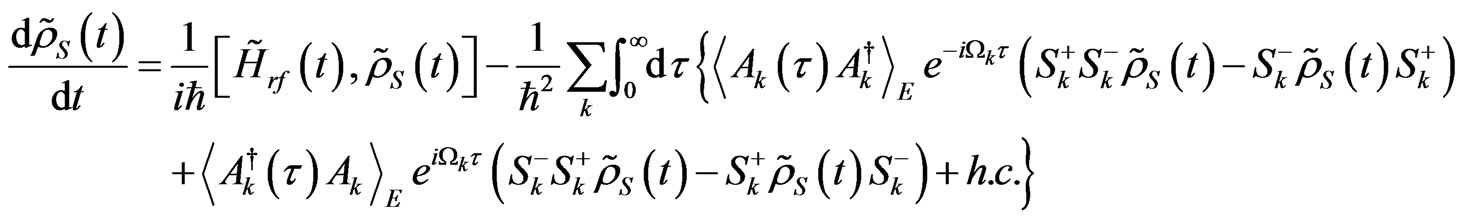
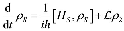
 (22)
(22)
where we have made the change of variables  with
with  such that
  and divided all by
 . The first term in the right hand side of (22) describes the ideal part of the dynamics in the interaction picture (von Neuman evolution), and the second part describes the open dynamics.
For a thermalized mixed environmental system one can sees that  then by doing typical calculations consisting in integrating over
  by using the spectral representation of the
 , performing the wave rotating approximation and regrouping terms, it follows that
 (23)
(23)
where the limit  has been taken, the superior limit in the integrals has been put infinity since the correlation functions decay exponentially in time, and the following definitions have been made
 (24)
(24)
The coefficients  and
and  are related to the coupling of the central system with the environment and depends on the characteristic frequencies of the modes in the neighborhood of each spin. The correlation functions are described by the Fourier transform of certain spectral density,
  , associated to the continuous modes in the thermal bath,
 (25)
(25)
with . The correlation functions can be written as
 (26)
(26)
where we get the operators
 (27)
(27)
being P.V. the Cauchy principal value. These operators are diagonal on the above basis, 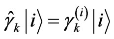 for example, and their eigenvalues are denoted with an upper index (see Appendix).
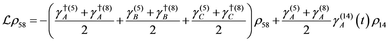
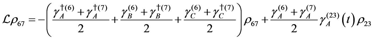
By regrouping terms in (23) and going back to Schrödingers picture, we obtain the following master equation
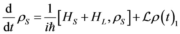 (28)
(28)
with  defined as
 (29)
(29)
where  are the matrix elements of the initial reduced density matrix operator, and
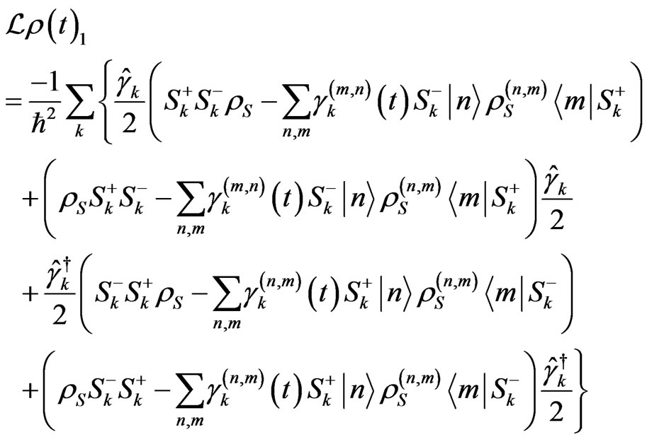
  in Equation (28) is given by
 (30)
(30)
which represents a Lamb shift Hamiltonian and can be not considered in the dynamics since it commutes with the entire  of the central system. In addition, it only generates a global shift in the spectrum. The time dependent coefficients are explicitly given by
 (31)
(31)
and they represent local phases for the non diagonal terms of the equations of the density matrix. Therefore, the positiveness and trace equal 1 are still satisfied for the density matrix. These phases depend linearly on the Ising coupling constants and bring about the quasi nonMarkovian behavior of the system.
If we consider low Ising coupling with respect the Larmor frequencies, then we can make the following approximation
 (32)
(32)
and (28) takes the following form
 (33)
(33)
where the term  is given by
 (34)
(34)
with the coefficients  and
and  written as
 (35)
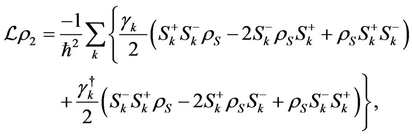
(35)
This type of master equations generates no-correlated thermalized cases which describes spontaneous and thermally induced emission-absorption process [3,28,29]. The environment generates excitations or de-excitations in the closed system by absorbing-emitting photons of the thermal bath. In this work, we want to establish the differences between Equation (28) which may describe a quasi-non-Markovian process via the oscillating term in the non diagonal elements of the dissipator, and Equation (33), which is the typical Markovian master equation for a system immerse in a bosonic field.
4. Physical Quantities
Let us considered a thermal bath of radiation modes at a temperature T. The environmental density matrix is given by
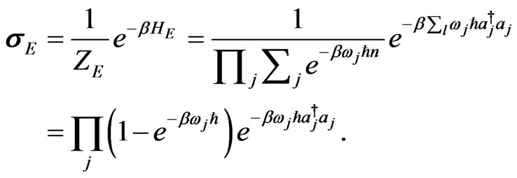 (36)
(36)
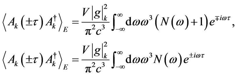
The interaction Hamiltonian between the central system and the environment is represented by a coupling between the polarization operator and a bosonic modes operators. The correlation functions involved in the system 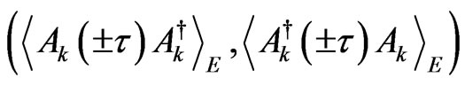 are calculated,
 (37)
(37)
The sum over i is dense (there are an uncountable number of radiation modes). If the volume containing this modes is large enough, we can go from a discrete distribution to a continuous distribution of the characteristic frequencies of the radiation modes. The number of characteristic frequencies with wave vector components f in the interval  in the volume V is given by
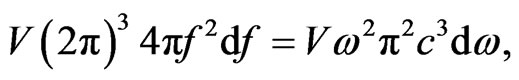 (38)
(38)
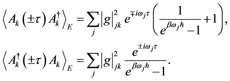
where . Thus the sum in the correlation functions can be changed by an integration over de frequencies with the proper weight factor,
 (39)
(39)
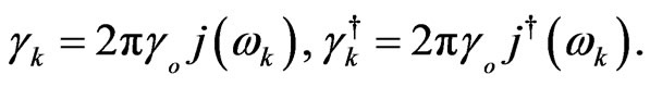
where we have taken a linearly dependence on the characteristic frequencies of the radiation modes,
 , and the Planck’s distribution function,
 (40)
(40)
Comparing this results with the definitions in (26) and (27), one can sees that
 (41)
(41)
and
 (42)
(42)
Once we get the definitions of all these constants, we can proceed to solve the above equations. The evolution equations of the matrix elements are given in appendix.
5. Simulations and Results
Our registers are made up of three qubits  with
with , or written them with decimal notation,
  ,
,  and so on. The parameters used for our simulation are taken from [25] regarding the Larmor frequencies of the nuclear spins and we take a higher Ising coupling strength for modelling the differences between the Markovian and the quasi-non Markovian regime but maintaining the
  method [25]. These parameters are (in units of
 ) as
) as
 (43)
(43)
There is still one free parameter which is the strength of the coupling between the environment and the central system . This will allow us to model high or low dissipation rates of a homogeneous or inhomogeneous environments. We take the assumption that the environment is acting homogeneously on each qubit, that is, there is a set of baths of characteristic frequencies affecting more closely the resonant frequencies of each spin.
The reduced density matrix is then made up of  complex elements, and if the initial state is always taken as the exited state
 , this means that the initial reduced density matrix has the values
  and
and  for
for .
.
5.1. Controlled-Not (CNOT) Quantum Gate
To get the CNOT quantum gate starting from the ground state , one applies a
  -pulse between this state and the state
 , with resonant frequency
 , to get the superposition state
 . Then, one applies a resonant
  -pulse between the states
  and
and , with resonant frequency
 , to get the final desired state
  which means that the expected CNOT density matrix would be such that
 , and all the other elements are equal to zero. In addition, one allows the system to have two and a half more resonant
  -pulses to have a better look of the CNOT behavior.
5.2. Dynamics at Room Temperature
We start modeling the dynamics by considering that the environment is at room temperature ( Kelvins). This assumption will make the system to evolve into a thermalized mixed state. We present in the following figures the differences of the behavior of the diagonal terms and the coherent terms involved in the CNOT quantum gate.
Figure 1 shows the behavior of the diagonal elements of the CNOT gate for low  and high
 dissipation rates (the high dissipation rate is still in the limit of considering the approximation of a perturbation of the central system) for the Markovian and semi(quasi)-non Markovian regimes at a temperature
 . We can see that the differences between them are very small but still distinguish. For each case, Markovian and quasi-non Markovian, the environment will lead the central system into a thermalized mixture states, with a thermalization time depending on the coupling constant with the environment. We need to point out that this difference increases as the spin coupling constant a first neighbor increases its value.
Figure 2 shows the behavior of the coherent terms involved in the CNOT gate. We can see that for high dissipation rates a fast thermalization of the system, making the coherent terms goes to zero very rapidly. The term  is related to the first pulse which makes the super-
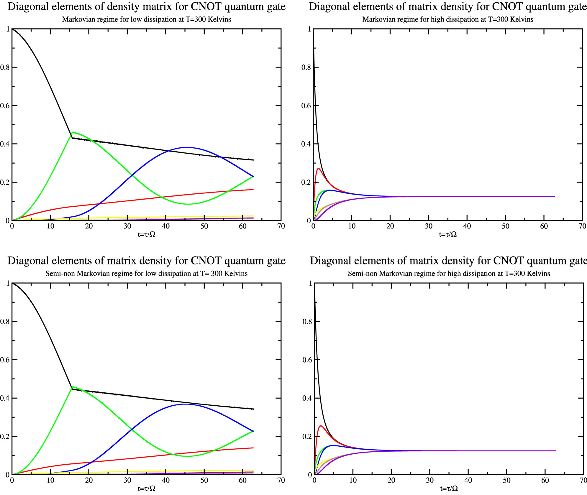
Figure 1. Diagonal elements of the density matrix for the CNOT quantum gate for low (left) and high (right) rates of dissipation in the Markovian and quasi-non Markovian regime at T = 300 Kelvins.
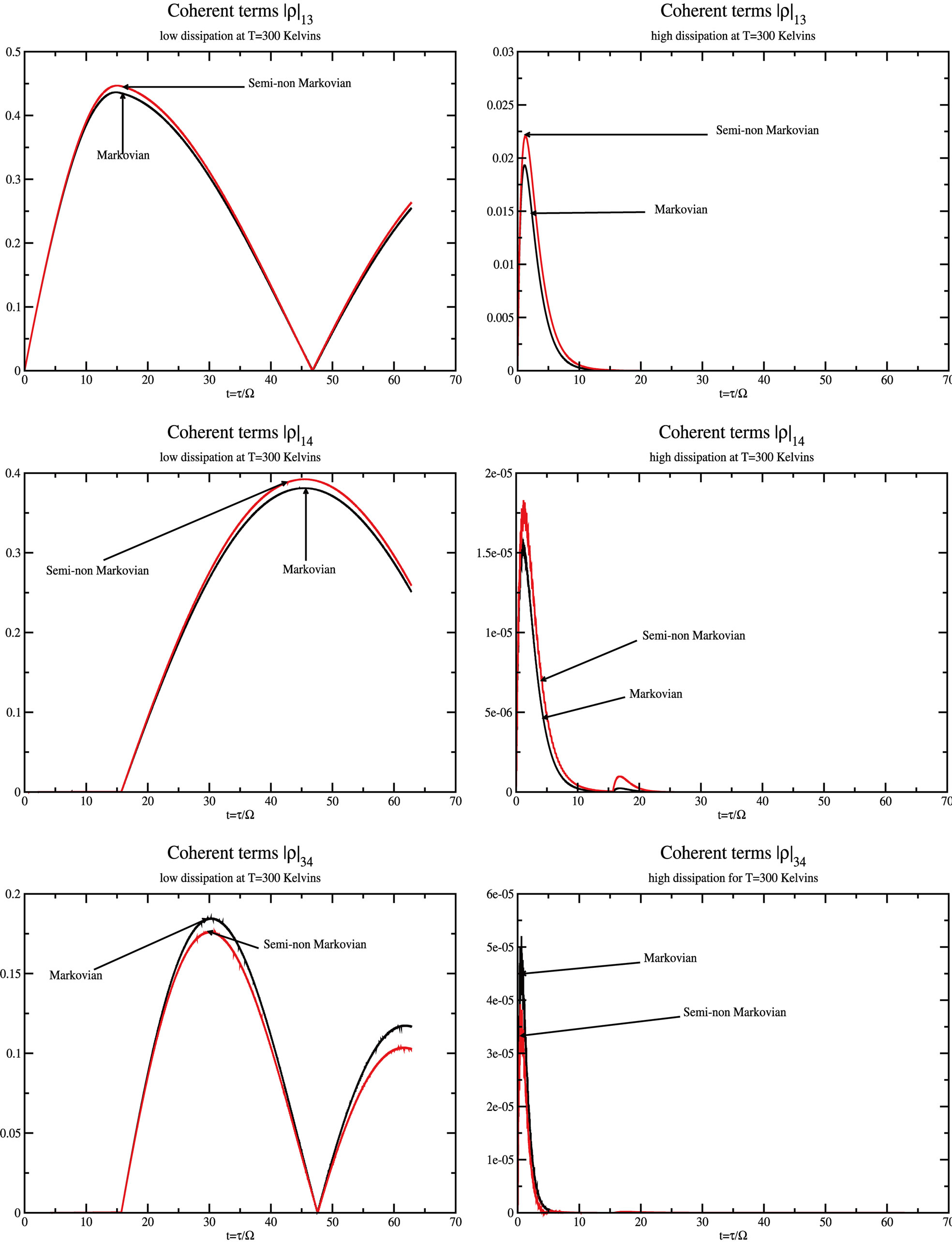
Figure 2. Coherent elements ,
,  and
and  of the density matrix for the CNOT quantum gate for low (left) and high (right) rates of dissipation in the Markovian and quasi-non Markovian regime at T = 300 Kelvins.
position state for the CNOT formation. Therefore, it has higher amplitude, since it will take some time for the environment to completely thermalize the whole system. For the last  -pulse for the CNOT formation, we see that the decoherence is already high. There is a very small sudden birth of coherence in the term
 , due to the pulses of the magnetic field needed to perform the quantum gate. For the high dissipation cases
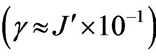 , the quasi-non Markovian and the Markovian regime are very similar, contrary to the low dissipation rate which even when it is less notorious, the difference in their amplitude is higher since decoherence is not strong. The elements involving the higher energy level
  their amplitude seem to have a grater amplitude for the quasi-non Markovian regime than in the Markovian regime. This situation is contrary in the element
 .
.
5.3. Dynamics at the Thermal Vacuum
At  Kelvins, the master equation takes the form as described in [28] for the A-Independent environment cases, and we still have the time dependent terms on the non diagonal elements of the master equation, referring to the quasi-non Markovian case. Figure 3 shows the behavior of the diagonal elements of the CNOT quantum gate at
  Kelvins. We can not see a distinguished difference between the Markovian and quasi-non Markovian regimes as we did in Figure 1. However, at high dissipation rate, we still seen for both cases (Markovian and quasi-non Markovian), the rise of the equilibrium ground state at the end of the whole process. This happens because our initial state is the most exited state, and during the process of dissipation, the environment is not giving off any energy to the system, the quantum system will deliver the energy to all the other states, exiting them. Therefore, by dissipation, all of them go back to zero, leaving the system in the ground state
  (purple curve in the figures).
Figure 4 shows the behavior of the coherent terms of
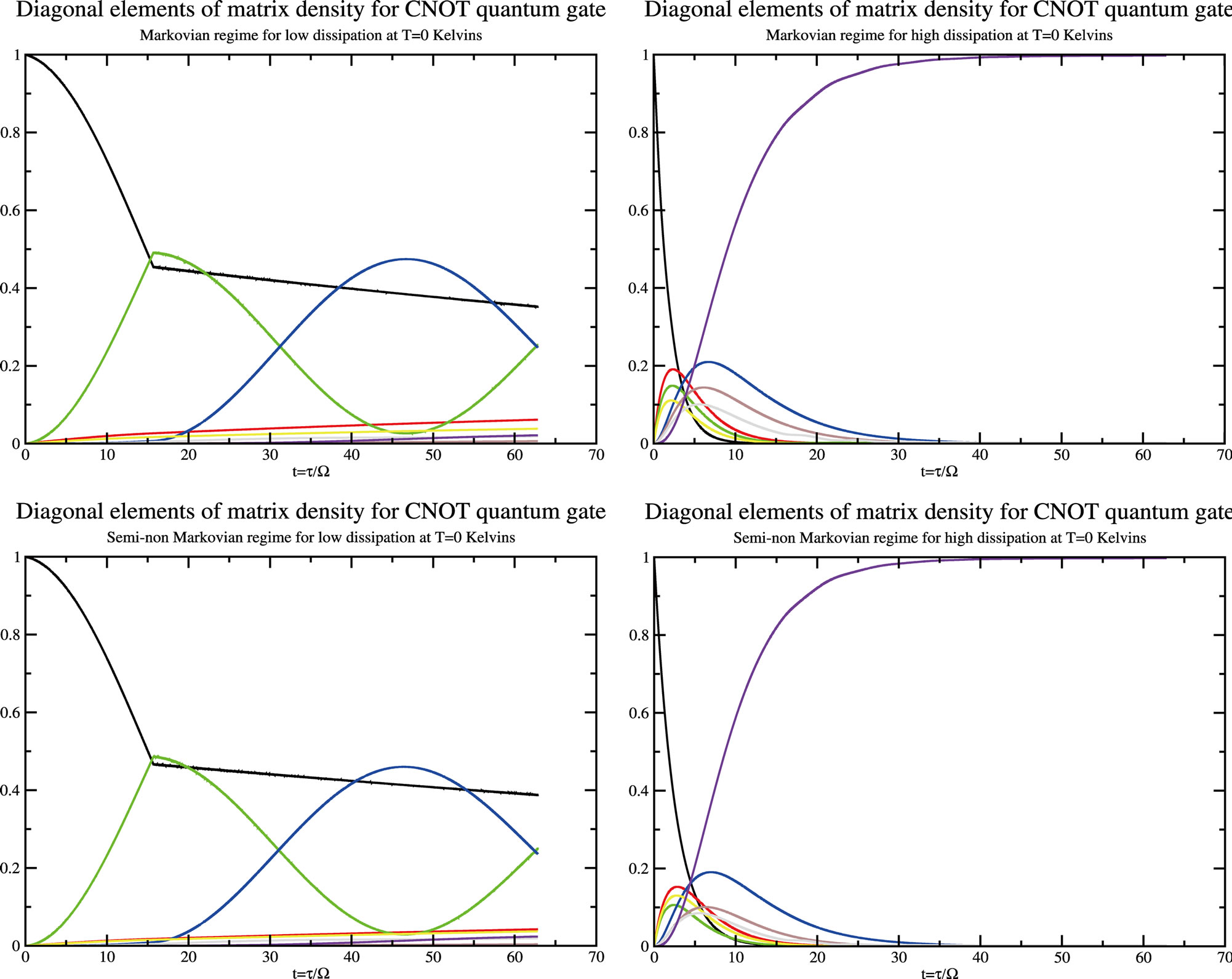
Figure 3. Diagonal elements of the density matrix for the CNOT quantum gate for low (left) and high (right) rates of dissipation in the Markovian and quasi-non Markovian regime at T = 0 Kelvins.
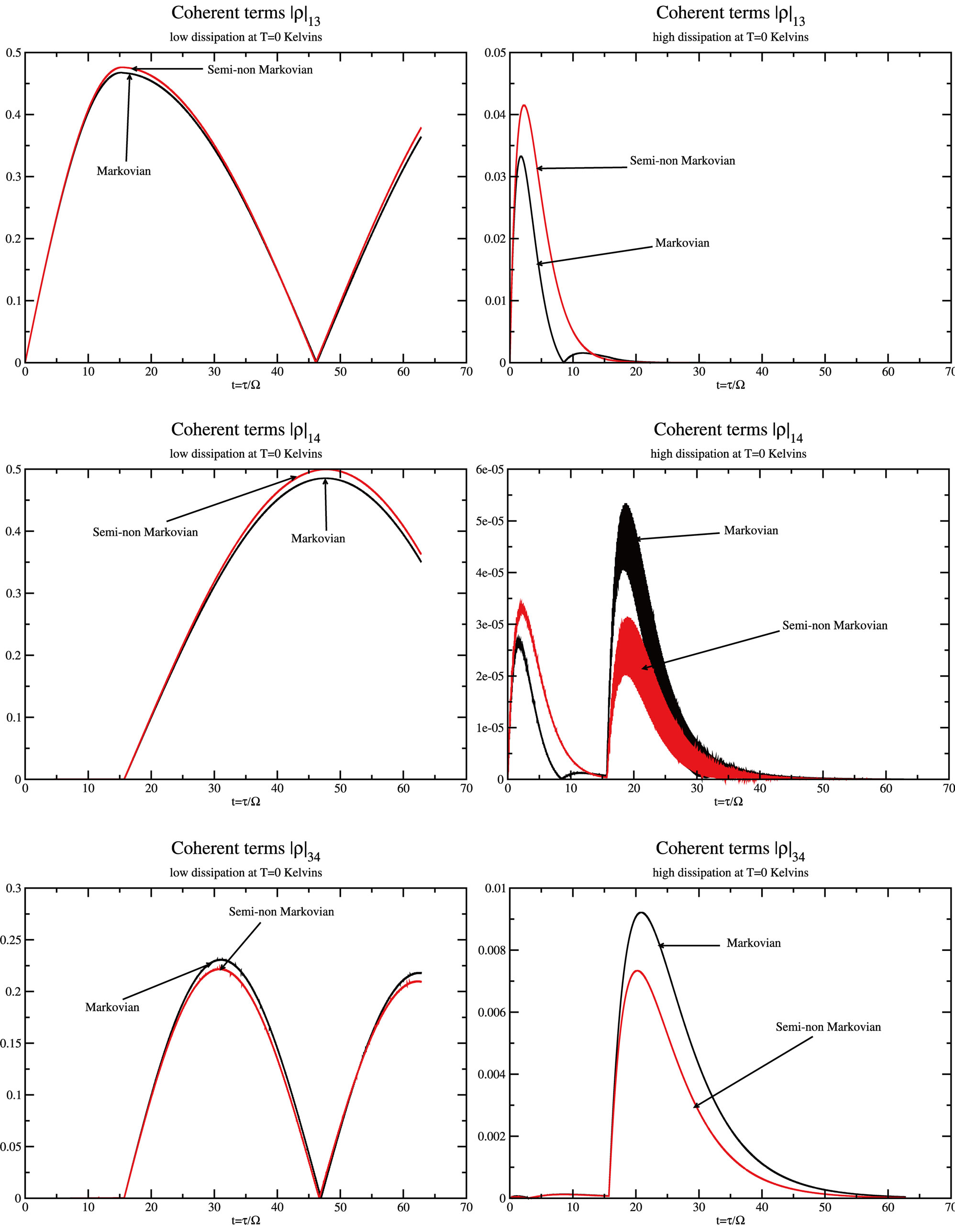
Figure 4. Coherent elements ,
,  and
and  of the reduced density matrix for low (left) and high (right) rates of dissipation in the Markovian and quasi-non Markovian regime at T = 0o K.
the reduced density matrix at . For low dissipation rates
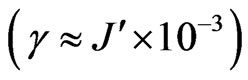 , we see a similar behavior as in the room temperature cases. For high dissipation rates
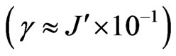 , we see less significant differences between the Markovian and the quasi-non Markovian cases, suggesting that this effect could be observable experimentally at low rates of dissipation.
5.4. Purity Calculations
The purity function, 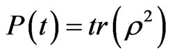 , is a measure of how close a quantum system is from its description as a pure state quantum system (the density matrix be written in term of a wave function
 ) and varies between 1 and 1/d (d the dimensionality of the density matrix). This function may decay with the decoherence since the system may move away from an initial pure state. Therefore, this function can be used to characterize the environment.
Figure 5 shows the behavior of the purity for the CNOT gate at room temperature and at . At room temperature it is observed a thermalization of the system, and at
  a recovery of the purity since the system goes to the quantum ground state, depending on the dissipation rate.
6. Conclusions
Within the weak coupling approximation for the study of quantum discrete system with environment, we have obtained a quantum master equation with a time dependent non diagonal dissipative coefficients which shows a quasi-non Markovian behavior. We have solved numerically the master equation for the reduced density matrix associated to our linear chain of three nuclear spin system interacting with the environment. We have made the
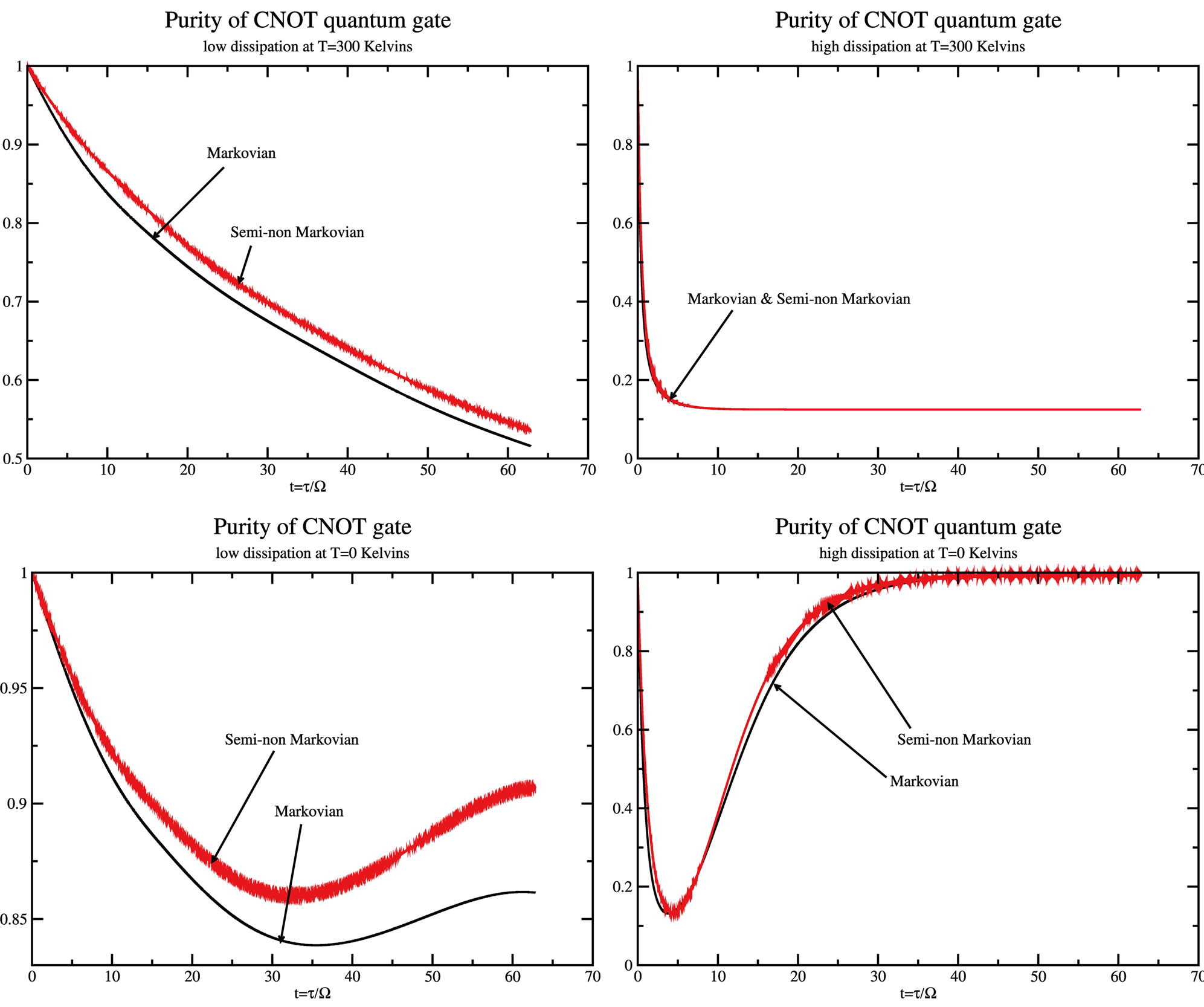
Figure 5. Purity for the Markovian and quasi-non Markovian regimes at T = 300 and T = 0 Kelvins for low (left) and hight (right) dissipation rates.
simulation of CNOT quantum gate operating in this dissipative environment and within the validity of this approximation. We have study the behavior of system-environment interaction with this quasi-non Markovian master equation and compared the results with the Markovian counterpart. The decoherence of this quantum logic gate have been determined, and we have seen a different behavior of the decoherence with the quasi-non Markovian and with Markovian master equations.
This difference between quasi-non Markovian and Markovian approaches on the reduced density matrix elements grows with the dissipation coefficients defined in the master equations, but the diagonal elements remain almost identical over the two types of process. Therefore, for high dissipation the measuring apparatus will not bring any information of the environmental interaction for a Markovian or quasi-non Markovian process, and for low dissipation this difference can, in principle, be measure. In addition, this difference must increase as the spin coupling parameter a fist neighbor increases since the spectrum becomes much more well defined. This comparison was also made using the purity parameter. For strong dissipation at  Kelvins, we found that purity may increase because, the condition
  on the density matrix, and this implies excitation of the equilibrium state involved in the dynamics (ground state), causing the system to try to return to a pure quantum state description.
REFERENCES
- G. López, M. Murgua and M. Sosa, “Quantization of One-Dimensional Free Particle Motion with Dissipation,” Modern Physics Letters B, Vol. 15, No. 22, 2001, pp. 965-971. doi:10.1142/S0217984901002750
- G. López and P. López, “Velocity Quantization Approach of the One-Dimensional Dissipative Harmonic Oscillator,” International Journal of Theoretical Physics, Vol. 45, No. 4, 2006, pp. 734-742. doi:10.1007/s10773-006-9064-9
- H.-P. Breuer and F. Petruccione, “The Theory of Open Quantum Systems,” Oxford University Press, Oxford, 2006.
- G. Lindblad, “On the Generators of Quantum Dynamical Semigroups,” Communications in Mathematical Physics, Vol. 48, No. 2, 1976, pp. 119-130. doi:10.1007/BF01608499
- A. O. Caldeira and A. T. Legget, “Path Integral Approach to Quantum Brownian Motion,” Physica A, Vol. 121, No. 3, 1983, pp. 587-616. doi:10.1016/0378-4371(83)90013-4
- B. L. Hu, J. P. Paz and Y. Zhang, “Quantum Brownian Motion in a General Environment: Exact Master Equation with Nonlocal Dissipation and Colored Noised,” Physical Review D, Vol. 45, No. 8, 1992, pp. 2843-2861. doi:10.1103/PhysRevD.45.2843
- J. P. Paz and W. H. Zurek, “Environment-Induced Decoherence, Classicality and Consistency of Quantum Histories,” Physical Review D, Vol. 48, 1993, pp. 2728-2738. doi:10.1103/PhysRevD.48.2728
- A. Rivas, A. D. K. Plato, S. F. Huelga and M. B. Plenio, “Markovian Master Equations: A Critical Study,” New Journal of Physics, Vol. 12, 2010, Article ID: 113032. doi:10.1088/1367-2630/12/11/113032
- W. H. Zurek, “Decoherence, Einselection, and the Quantum Origins of the Classical,” Reviews of Modwen Physics, Vol. 75, 2003, pp. 715-775.
- W. H. Zurek, “Decoherence and the Transition from Quantum to Classical,” arXiv: quant-ph/0306072, 2003, pp. 1-24.
- H. D. Zeh, “There Is Not ‘First’ Quantization,” Physical Letters A, Vol. 309, No. 5, 2003, pp. 329-334. doi:10.1016/S0375-9601(03)00209-3
- M. Zwolak, H. T. Quan and W. H. Zurek, “Quantum Darwinism in a Mixed Environment,” Physical Review Letters, Vol. 103, 2009, Article ID: 110402. doi:10.1103/PhysRevLett.103.110402
- L. Mazzola, J. Piilo and S. Maniscalco, “Sudden Transition between Classical and Quantum Decoherence,” Physical Review Letters, Vol. 104, No. 20, 2010, Article ID: 200401. doi:10.1103/PhysRevLett.104.200401
- F. Intravaia, S. Maniscalco and A. Messina, “DensityMatrix Operatorial Solution of the Non-Markovian Master Equation for Quantum Brownian Motion,” Physical Review A, Vol. 67, No. 4, 2003, Article ID: 042108. doi:10.1103/PhysRevA.67.042108
- S. Maniscalco and F. Petruccione, “Non-Markovian Dynamics of a Qubit,” Physical Review A, Vol. 73, No. 1, 2006, Article ID: 012111. doi:10.1103/PhysRevA.73.012111
- H.-P. Breuer, “Non-Markovian Generalization of the Lindblad Theory of Open Quantum Systems,” Physical Review A, Vol. 75, No. 2, 2007, Article ID: 022103. doi:10.1103/PhysRevA.75.022103
- H.-P. Breuer, E.-M. Laine and J. Piilo, “Measure for the Degree of Non-Markovian Behavior of Quantum Processes in Open Systems,” Physical Review A, Vol. 103, No. 21, 2009, Article ID: 210401.
- A. Rivas, S. F. Huelga and M. B. Plenio, “Entanglement and Non-Markovian of Quantum Evolutions,” Physical Review Letters, Vol. 105, No. 5, 2010, Article ID: 050403. doi:10.1103/PhysRevLett.105.050403
- G. P. Berman, D. D. Doolen, D. I. Kamenev, G. V. López and V. I. Tsifrinovich, “Perturbation Theory and Numerical Modeling of Quantum Logic Operations with Large Number of Qubits,” Contemporary Mathematics, Vol. 305, 2002, pp. 13-41. doi:10.1090/conm/305/05213
- D. Solenov, D. Tolkunov and V. Privman, “Exchange Interaction, Entanglement, and Quantum Noise Due to Thermal Bosonic Field,” Physical Review B, Vol. 75, No. 3, 2007, Article ID: 035134. doi:10.1103/PhysRevB.75.035134
- A. A. Slutskin, K. N. Bratus, A. Bergvall and V. S. Shumeiko, “Non-Markovian Decoherence of a Two-Level System Weakly Coupled to a Bosonic Bath,” Europhysics Letters, Vol. 96, No. 4, 2011, Article ID: 40003. doi:10.1209/0295-5075/96/40003
- N. P. Oxtopy, A. Rivas, S. F. Huelga and R. Fazio, “Probing a Composite Spin-Boson Environment,” New Journal of Physics, Vol. 11, 2009, Article ID: 063028.
- G. V. López and L. Lara, “Numerical Simulation of a Controlled-Controlled-Not (CCN) Quantum Gate in a Chain of Three Interacting Nuclear Spins System,” Journal of Physics B: Atomic, Molecular and Optical Physics, Vol. 39, No. 18, 2006, pp. 3897-3904. doi:10.1088/0953-4075/39/18/019
- G. V. López, J. Quezada, G. P. Berman, D. D. Doolen, and V. I. Tsifrinovich, “Numerical Simulation of a Quantum Controlled-Not Gate Implemented on Four-Spin Molecules at Room Temperature,” Journal of Optics B: Quantum and Semiclassical Optics, Vol. 5, No. 2, 2003, pp. 184-189. doi:10.1088/1464-4266/5/2/311
- G. V. López, T. Gorin and L. Lara, “Simulation of Grover’s Quantum Search Algorithm in an Ising-Nuclear-SpinChain Quantum Computer with First-and-Second-Nearest-Neighbor Couplings,” Journal of Physics B: Atomic, Molecular and Optical Physics, Vol. 41, No. 5, 2008, Article ID: 055504.
- N. Y. Yao, et al., “Scalable Architecture for a Room Temperature Solid-State Quantum Information Processor,” arXiv: 1012.2864v1, 2002.
- F. W. Cummings, “Stimulated Emission of Radiation in a Single Mode,” Physical Review Letters, Vol. 140, No. 4A, 1965, p. A1051.
- G. V. López and P. López, “Study of Decoherence of Elementary Gates Implemented in a Chain of Few Nuclear Spins Quantum Computer Model,” Journal of Modern Physics, Vol. 3, No. 1, 2012, p. 85.
- S. Das and G. S. Agarwal, “Decoherence Effects in Interacting Qubits under the Influence of Various Environments,” Journal of Physics B: Atomic, Molecular and Optical Physics, Vol. 42, 2009, Article ID: 205502.
Appendix
The evolution equation for the density matrix elements are given from Equation (28) by
 (X1)
(X1)
Making the following definition
 (X2)
(X2)
one gets
Von Neuman  Part
Part
 (V1)
(V1)
 (V2)
(V2)
 (V3)
(V3)
 (V4)
(V4)
 (V5)
(V5)
 (V6)
(V6)
 (V7)
(V7)
 (V8)
(V8)
 (V9)
(V9)
 (V10)
(V10)
 (V11)
(V11)
 (V12)
(V12)
 (V13)
(V13)
 (V14)
(V14)
 (V15)
(V15)
 (V16)
(V16)
 (V17)
(V17)
 (V18)
(V18)
 (V19)
(V19)
 (V20)
(V20)
 (V21)
(V21)
 (V23)
(V23)
 (V24)
(V24)
 (V25)
(V25)
 (V26)
(V26)
 (V27)
(V27)
 (V28)
(V28)
 (V29)
(V29)
 (V30)
(V30)
 (V31)
(V31)
 (V32)
(V32)
 (V33)
(V33)
 (V34)
(V34)
 (V35)
(V35)
 (V36)
(V36)
 (V37)
(V37)
Dissipation Part


Eigenvalues of the  Operator
The eigenvalues equation is written as , for a three nuclear spins
 . The basis is taken in decimal notation, like
 ,
,  , and so on.
 (A1)
(A1)
 (A2)
(A2)
 (A3)
(A3)
 (A4)
(A4)