ABSTRACT

In this study, we establish an approximate method which produces an approximate Hermite polynomial solution to a system of fractional order differential equations with variable coefficients. At collocation points, this method converts the mentioned system into a matrix equation which corresponds to a system of linear equations with unknown Hermite polynomial coefficients. Construction of the method on the afore- mentioned type of equations has been presented and tested on some numerical examples. Results related to the effectiveness and reliability of the method have been illustrated.

Keywords:

Fractional Order Differential Equations, Hermite Polynomials, Hermite Series, Collocation Methods

1. Introduction

As cited in [1] [2] [3] , fractional order differential equations can be considered as a generalization of integer order ones and it is approved that the mathematical modelling on physical processes naturally leads to differential equations for fractional order. Consequently, applications of fractional differential equations appear very frequently in many fields, such as engineering, physics, finance, chemistry and bioengineering [1] [2] [4] [5] [6] . Unfortunately, the resulting model equations are usually difficult to solve analytically. Therefore, it is vital to develop some numerical or approximate techniques. Nowadays, the studies on fractional order differential equations and their solutions have become very popular and attracted the attention of many researchers. So far many numerical or approximate schemes have been developed. Among them, finite difference approximation methods [7] [8] [9] [10] , fractional linear multistep methods [11] [12] [13] , quadrature formula approach [14] , the Adomian decomposition method [15] [16] [17] , variational iteration method [17] [18] [19] , and differential transform method [20] [21] can be accounted. For some class of fractional order differential equations polynomial approximation methods were also given by Kumar and Agarwal and the references can be found in [22] [23] [24] .

So far, a lot of works published on fractional order linear/non-linear differential equations but there are still works have to be done. In this work, we aim to extend the Hermite Collocation method (HCM) for obtaining solution to a system of fractional order differential equations with variable coefficients and specified initial conditions. The technique constructs an analytical solution of the form of a truncated Hermite series with unknown coefficients. The orthogonal Hermite polynomials have the importance in the theory of light fluctuations and quantum states and, in particular, some problems of coastal hydrodynamics and meteorology [25] . This method is the adaptation of Taylor collocation method with Hermite polynomials and first has been used to solve higher-order linear Fredholm integro differential equation in [26] and the development of the method can be found in [26] .

This paper is organized as follows. Section 2 involves some basic definitions and properties of fractional calculus. In Section 3, the theory and definitions of Hermite collocation method and the construction of this method for fractional order systems are presented. In Section 4, the matrix relations for initial conditions are defined and the Section 5 deals with the error estimate for the method. Section 6 involves some illustrative examples. Finally, the last section concludes with some remarks based on the reported research.

2. Preliminary and Notations

We first recall the following known definitions and preliminary facts of fractional derivatives and integrals which are used throughout this paper.

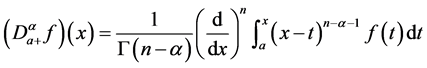
Definition 2.1. ( [1] [27] ) Let. The Riemann Liouville fractional integral of a function f of order is defined by

where is the gamma function and. For consistency, we take, which is identity operator and holds.

Definition 2.2. ( [1] [27] ) The Riemann Liouville fractional derivative of order of a function f is defined by

(1)

where and is defined as the integer part of. Again, for consistency, , then, it follows where.

Alternatively, we recall the following definition of Caputo ( [28] ) for fractional derivatives and Caputo’s definition is much more suitable for identifiable physical states, i.e. initial or boundary conditions. Therefore, all derivatives will be in Caputo sense throughout the paper.

Definition 2.3. The Caputo fractional derivative of order of a function f on an interval is defined by

(2)

Some properties of Caputo derivative are given as follows:

1) ( [1] ) Let and or then

2) ( [1] ) Let and. If or, then

3) ( [29] ) For every

4) Let and for some then,

(3)

3. Establishing Hermite-Collocation Method for Fractional Order Systems with Variable Coefficients

In this section, we will consider the following system of fractional order differential equations (FDEs) with variable coefficients, ,

(4)

where and, are continuous functions on. The initial conditions are defined as

(5)

In Equation (5), are some given constants and we denote for simplicity. Here, we assume that the approximate solution of the problem is given in terms of truncated Hermite series,

(6)

where defines the unknown Hermite coefficients of the solution and N is a positive integer which is chosen sufficiently small for avoiding the laborious work such that. Therefore, the fundamental matrix relation of Equation (4) can be written as

(7)

where and are defined as follows:

Now, we need to define the Caputo derivatives of . By using Equation (6), therefore, we write (see [26] ),

(8)

where and are defined as and respectively. Now, we will describe the matrix representation of the truncated Hermite series in terms of rational power of the indepandant variable x, by using the following generalized formula:

where and Now, in terms of N being odd or even, we denote the truncated series in matrix notation such as follows (see [26] ):

If N is an odd number:

(9)

if N is even then,

(10)

Hence, we have or equivalently,

(11)

and letting,

and then, substitution of Equation (11) into Equation (6) yields,

(12)

Now, the nath order Caputo derivative of Equation (12) is written as

(13)

or equivalently:

(14)

Here, the matrix B is defined as follows ():

Hence, if we substitute Equation (14) into Equation (13) we have:

(15)

Therefore, the matrices in Equation (15), for, are clearly shown by

where the each submatrix, consisting of rows and columns. Consequently, the above matrix equation can be written as,

(16)

where appears as consisting of k rows and columns. Hence, inserting the collocation points, , , into Equation (7) then, we have

(17)

where and G are of the form:

,

Apart from this, arranging Equation (16) for each collocation points then, we can write explicitly as,

Therefore, the matrix form is equivalent to

(18)

where

,

and each submatrix in is denoted by,

Consequently, now we denote Equation (7) of the form:

(19)

Then, by writing Equation (18) in Equation (19), the matrix form of the system of FDEs is written by

(20)

Moreover, denoting

hence, the system of FDEs is simply shown by

(21)

Now, Equation (21) constructs an algebraic system. To obtain the solution of the above system, the augmented matrix is written as follows:

(22)

Solving the above system, as a result, we obtain the desired Hermite coefficients in the truncated Hermite series. Hence, writing in Equation (12) we evaluate the unknowns of the system of FDEs (Equation (4)).

4. Matrix Relations for Initial Conditions

In generally, we look for the solution of the system of FDEs under specified conditions. However, preceding calculations do not involve these conditions. Therefore, we need to incorporate these conditions into the work. Then, we have to establish the new form of Equation (22) which involves initial conditions, Equation (5). Now, we start by writing Equation (5) explicitly for each same as below:

Hence, by using the above relations, we obtain t-conditions for each unknown,. For example, for we obtain t conditions such as follows:

Therefore, the conditions in matrix notation fulfils,

(23)

where

and for, we define

.

Now writing Equation (16) into Equation (23) for, we obtain

(24)

Now, calling U as,

then, the Hermite polynomial coefficients matrix which corresponds to the given initial conditions (Equation (5)), can be written as

(25)

In Equation (25), U involves kt rows and columns. Consequently, deleting rows in Equation (21) and then replacing these rows by Equation (25), we obtain the whole augmented matrix of the system, , as follows:

(26)

Hence, the system of algebraic equations of which unknowns are the hermite polynomial coefficients are shown by

(27)

Theorem 1. If, (i.e.) then,

(28)

By the above theorem, the matrix of Hermite coefficients, A is uniquely determined by Equation (27). Finally, substitution of these coefficients into the truncated Hermite series gives the desired solution of the form:

(29)

5. Error Estimate for the Solution

The truncated Hermite series, Equation (29), is the approximate solution of Equation (4) with the given initial conditions, (Equation (5)). Since this solution should approximately satisfy the Equation (4) hence, the residuals

give the error at the particular points ,. Let us now denote the residuals by as an error function. The error should be approximately zero or where is any positive constant. If the is prescribed before then, the truncation limit for N is increased until becomes smaller than (see [21] [26] ).

6. Numerical Applications

The technique which we have developed to solve fractional order systems is quite feasible and accurate. To show the accuracy of the method the following system of FDEs with variable coefficients are solved. All the numerical calculations have been performed by using MatlabR2007b.

Example 6.1. We first consider the problem, which is mentioned in [16] (),

(30)

with given initial conditions,

(31)

Now, we will look for a solution to the system of FDEs in terms of Hermite polynomials of the form;

Here, we will take into consideration:. Since and, then it requires that. As it should be, therefore, we can select for convenience. Now, Equation (4) can be rewritten as:

(32)

By using Equations ((6) and (20)) then, the matrix form of the system, Equation (30), is written by

(33)

where, , , , , , , and the rest are zero. From here, we evaluate that. Hence, the matrix form of the Equation (30) is deduced as,

(34)

For, the collocation points are and. Then the matrices in Equation (34) become,

Hence, we have

Therefore, evaluating Equation (34), we obtain W as,

(35)

then, the augmented matrix for the system, or, is obtained as,

(36)

where the matrix consisting of k rows and columns and similarly, the matrix form of the initial conditions, Equation (31), is obtained from Equation (24) such as follows:

(37)

by defining,

Hence, we have,

Then, by substituting the related matrices into Equation (37), the augmented matrix is obtained as

(38)

Moreover, deleting the last two rows of Equation (36) and replacing the matrix in Equation (38), we have

(39)

Since then, the solution of the resulting linear system, gives coefficient matrix, which is equivalent to

In conclusion, writing these coefficients into:

(40)

we obtain the solutions of the system of FDEs as follows

(41)

(42)

Figure 1 shows the HCM solution of the system, Equation (30). Figure 2(a)) shows the Differential Transform solution and Figure 2(b)) Adomian Decomposition solution of the same system.

Example 6.2. In [30] , the authors have modeled the pollutant problem in a lake which connected by channels by the following fractional order system (see Figure 3),

(43)

where they considered:, and the initial conditions were de- fined as In [31] , the authors solved the following

ordinary system by Bessel Polynomial Collocation method (BCM) with the assumptions: and the initial conditions;

(44)

Now, we will solve the fractional form of Equation (44), which is defined as in Equation (44) by HCM method. We consider here the case: and. Since then, it requires that. As a result, we can choose. Therefore, the solution will be of the form:

The fundamental matrix form of the system of Equation (44) is obtained from Equations ((6) and (20)) such as follows,

(45)

which is equivalent to:

Then, by performing the calculations, we obtain the following matrices:

then, the agumented matrix is obtained at collocation points as follows:

Since, then, the coefficient matrix, is obtained. When these coefficients substituted into

the solution of the system, Equation (44), is obtained as follows;

Figure 4 shows the plots of and, which are the solutions of Example 6.2 respectively. In these plots, the results have been compared by BCM method and our method (HCM) for. Furthermore, each plots also shows the results for, which exists first time in the literature and there is a clear difference between the solution of the fractional order sytem and ordinary differential equation system although, there is a small change between.

7. Conclusion

The basic goal of this work is to employ HCM method to obtain solution for a system of fractional order differential equations. These types of systems with variable coefficients are usually difficult to solve analytically. However, the presented method provides considerable simplifications in the solution. The coefficients of truncated Hermite series can be evaluated easily by the help of any symbolic computer packages. The obtained results demonstrate the reliability of the algorithm and give us a wider applicability to fractional higher order systems.

Cite this paper

Pirim, N.A. and Ayaz, F. (2016) A New Technique for Solving Fractional Order Systems: Hermite Col- location Method. Applied Mathematics, 7, 2307-2323. http://dx.doi.org/10.4236/am.2016.718182

References

- 1. Kilbas, A.A., Sirvastava, H.M. and Trujillo, J.J. (2006) Theory and Application of Fractional Differential Equations. In: North-Holland Mathematics Studies, Vol. 204, Amsterdam.
- 2. Ross, B. (1975) Fractional Calculus and Its Applications. Lecture Notes in Mathematics, 457, 80-89.
https://doi.org/10.1007/BFb0067098 - 3. Oldham, K.B. and Spanier, J. (2006) The Fractional Calculus. Theory and Applications of Differentiation and Integration of Arbitrary Order. Dower, New York.
- 4. Stanislavsky, A.A. (2004) Fractional Oscillator. Physical Review E, 70, 051103.
https://doi.org/10.1103/PhysRevE.70.051103 - 5. Mainardi, F., Luchko, Y. and Pagnini, G. (2001) The Fundamental Solution of the Space-Time Fractional Diffusion Equation. Fractional Calculus and Applied Analysis, 4, 153-152.
- 6. Trujillo, J.J. (1999) On a Riemann-Liouville Generalised Taylor’s Formula. Journal of Mathematical Analysis and Applications, 231, 255-265.
https://doi.org/10.1006/jmaa.1998.6224 - 7. Ciesielski, M. and Leszcynski, J. (2003) Numerical Simulations of Anomalous Diffusion. Computer Methods Mech Conference, Gliwice Wisla Poland.
- 8. Yuste, S.B. (2006) Weighted Average Finite Difference Methods for Fractional Diffusion Equations. Journal of Computational Physics, 1, 264-274.
https://doi.org/10.1016/j.jcp.2005.12.006 - 9. Odibat, Z.M. (2006) Approximations of Fractional Integrals and Caputo Derivatives. Applied Mathematics and Computation, 178, 527-533.
https://doi.org/10.1016/j.amc.2005.11.072 - 10. Odibat, Z.M. (2009) Computational Algorithms for Computing the Fractional Derivatives of Functions. Mathematics and Computers in Simulation, 79, 2013-2020.
https://doi.org/10.1016/j.matcom.2008.08.003 - 11. Ford, N.J. and Joseph Connolly, A. (2009) Systems-Based Decomposition Schemes for the Approximate Solution of Multi-Term Fractional Differential Equations. Journal of Computational and Applied Mathematics, 229, 382-391.
https://doi.org/10.1016/j.cam.2008.04.003 - 12. Ford, N.J. and Charles Simpson, A. (2001) The Numerical Solution of Fractional Differential Equations: Speed versus Accuracy. Numerical Algorithms, 26, 333-346.
https://doi.org/10.1023/A:1016601312158 - 13. Sweilam, N.H., Khader, M.M. and Al-Bar, R.F. (2007) Numerical Studies for a Multi Order Fractional Differential Equations. Physics Letters A, 371, 26-33.
https://doi.org/10.1016/j.physleta.2007.06.016 - 14. Diethelm, K. (1997) An Algorithm for the Numerical Solution of Differential Equations of Fractional Order. Electronic Transactions on Numerical Analysis, 5, 1-6.
- 15. Momani, S. and Odibat, Z. (2006) Analytical Solution of a Time-Fractional Navier-Stokes Equation by Adomian Decomposition Method. Applied Mathematics and Computation, 177, 488-494.
https://doi.org/10.1016/j.amc.2005.11.025 - 16. Odibat, Z. and Momani, S. (2007) Numerical Approach to Differential Equations of Fractional Order. Journal of Computational and Applied Mathematics, 207, 96-110.
https://doi.org/10.1016/j.cam.2006.07.015 - 17. Odibat, Z. and Momani, S. (2008) Numerical Methods for Nonlinear Partial Differential Equations of Fractional Order. Applied Mathematical Modelling, 32, 28-39.
https://doi.org/10.1016/j.apm.2006.10.025 - 18. Odibat, Z. and Momani, S. (2006) Application of Variational Iteration Method to Equation of Fractional Order. International Journal of Nonlinear Sciences and Numerical Simulation, 7, 271-279.
https://doi.org/10.1515/IJNSNS.2006.7.1.27 - 19. Wu, J.L. (2009) A Wavelet Operational Method for Solving Fractional Partial Differential Equations Numerically. Applied Mathematics and Computation, 214, 31-40.
https://doi.org/10.1016/j.amc.2009.03.066 - 20. Ertürk, V.S. and Momani, S. (2008) Solving Systems of Fractional Differential Equations Using Differential Transform Method. Journal of Computational and Applied Mathematics, 215, 142-151.
https://doi.org/10.1016/j.cam.2007.03.029 - 21. Yalcnbas, S., Konuralp, A., Demir, D.D. and Sorkun, H.H. (2010) The Solution of the Fractional Differential Equation with the Generalized Taylor Collocation Method. International Journal of Research & Reviews in Applied Sciences, 4, 296-303.
- 22. Kumar, P. and Agrawal, O.P. (2006) An Approximate Method for Numerical Solution of Fractional Differential Equations. Signal Process, 86, 2602-2610.
https://doi.org/10.1016/j.sigpro.2006.02.007 - 23. Kumar, P. (2006) New Numerical Schemes for the Solution of Fractional Differential Equations. Southern Illinois University at Carbondale, Vol. 134.
- 24. Kumar, P. and Agrawal, O.P. (2006) Numerical Scheme for the Solution of Fractional Differential Equations of Order Greater than One. Journal of Computational and Nonlinear Dynamics, 1, 178-185.
https://doi.org/10.1115/1.2166147 - 25. Dattoli, G. (2004) Laguerra and Generalized Hermite Polynomials: The Point of View of the Operation Method. Integral Transforms and Special Functions, 15, 93-99.
https://doi.org/10.1080/10652460310001600744 - 26. Akgonüllü, N., Sahin, N. and Sezer, M. (2010) A Hermite Collocation Method for the Approximate Solutions of Higher-Order Linear Fredholm Integro-Differential Equations, Numerical Methods for Partial Differential Equations, 27, 1708-1721.
- 27. Podlubny, I. (1999) Fractional Differential Equations. Academic Press, New York.
- 28. Caputo, M. (1967) Linear Models of Dissipation Whose Q Is Almost Frequency Independent II. Geophysical Journal of the Royal Astronomical Society, 13, 529-539.
https://doi.org/10.1111/j.1365-246X.1967.tb02303.x - 29. Samko, S.G., Kilbas, A.A. and Marichev, O.I. (1993) Fractional Integrals and Derivatives: Theory and Applications. Gordon and Breach, Amsterdam.
- 30. Biazar, J., Shahbala, M. and Ebrahimi, H. (2010) VIM for Solving the Pollution Problem of a System of Lakes. Journal of Control Science and Engineering, 2010, Article ID: 829152.
https://doi.org/10.1155/2010/829152 - 31. Yüzbas, S., Sahin, N. and Sezer, M. (2012) A Collocation Approach to Solving the Model of Pollution for a System of Lakes. Mathematical and Computer Modelling, 55, 330-341.
https://doi.org/10.1016/j.mcm.2011.08.007