Applied Mathematics
Vol.07 No.17(2016), Article ID:72012,22 pages
10.4236/am.2016.717168
Computational Methods for Three Coupled Nonlinear Schrödinger Equations
M. S. Ismail, S. H. Alaseri
Department of Math, King Abdulaziz University, Jeddah, Kingdom of Saudi Arabia

Copyright © 2016 by authors and Scientific Research Publishing Inc.
This work is licensed under the Creative Commons Attribution International License (CC BY 4.0).
http://creativecommons.org/licenses/by/4.0/


Received: September 8, 2016; Accepted: November 12, 2016; Published: November 15, 2016
ABSTRACT
In this work, we will derive numerical schemes for solving 3-coupled nonlinear Schrödinger equations using finite difference method and time splitting method combined with finite difference method. The resulting schemes are highly accurate, unconditionally stable. We use the exact single soliton solution and the conserved quantities to check the accuracy and the efficiency of the proposed schemes. Also, we use these methods to study the interaction dynamics of two solitons. It is found that both elastic and inelastic collision can take place under suitable parametric conditions. We have noticed that the inelastic collision of single solitons occurs in two different manners: enhancement or suppression of the amplitude.
Keywords:
Three Coupled Nonlinear Schrodinger Equations, Finite Difference Method, Time Splitting Method, Interaction of Solitons

1. Introduction
In recent years, the concept of soliton has been receiving considerable attention in optical communications, since soliton is capable of propagating over long distances without change of shape and velocity. It has been found that the soliton propagating through optical fiber arrays is governed by a set of equations related to the coupled nonlinear Schrödinger equation [1] [2] .
 (1)
(1)
where ,
,  is the envelope or the amplitude of the jth wave packets. Equation (1) reduces to the standard nonlinear Schrödinger equation for
 , to Manakov integrable system for
 , and recently for this case the exact two soliton solution obtained and novel shape changing in elastic collision property has been brought out. The system for
  is of physical interest, in optical communication, and in bio- physics this system can be used to study the lunching and propagation of solitons along the three spines of an alpha-helix shape changing in protein [1] [2] [3] [4] . In this work, we are going to derive some numerical methods for solving the three coupled nonlinear Schrödinger equations (3-CNLS)
 (2)
(2)
 (3)
(3)
 (4)
(4)
with initial conditions
 (5)
(5)
and the homogenous boundary conditions

The exact solution of the 3-coupled nonlinear Schrödinger equation [1] [2] is given by
 (6)
(6)

where  are four arbitrary complex parameters. Further
  gives the amplitude of the jth mode and
  the soliton velocity.
Many numerical methods for solving the coupled nonlinear Schrödinger equation are derived in the last two decades. Finite difference and finite element methods are used to solve this system by Ismail [5] - [10] . A conservative compact finite difference schemes are given in [11] [12] . In [3] [4] , Xing Lü studied the bright soliton collisions with shape change by intensity for the coupled Sasa-Satsuma system in the optical fiber communications. A higher order exponential time differencing scheme for system of coupled nonlinear Schrödinger equation is given in [13] . A semi-explicit multi-sypm- lectic splitting scheme for 3-coupled nonlinear Schrödinger equation is given in [14] . Many researchers are used time splitting method for solving the coupled non-linear schrödinger equation, the basic idea in this method is to split the original system into a linear subsystem and nonlinear subsystem, The splitting simplify the problem, since the linear problem is uncoupling, relatively easy to solve and the nonlinear problem can be solved exactly due to their point-wise conservation law, for more details see [15] - [23] .
To avoid complex computations we assume
 (7)
(7)
where  are real functions, the systems (2)-(4) can be written as
 (8)
(8)
 (9)
(9)
 (10)
(10)
where
 (11)
(11)
The resulting systems (8)-(10) can be written in a matrix-vector form as
 (12)
(12)
where

Proposition 1 The three coupled nonlinear Schöridinger equations have the con- served quantities
 (13)
(13)
 (14)
(14)
 (15)
(15)
Proof : we consider the first conserved quantity (13), from (8) we have
 (16)
(16)
 (17)
(17)
by multiplying (16) by  and (17) by
  and by adding the resulting equ- ations to obtain
 (18)
(18)
By integrating Equation (18) with respect to x from  to
to  and using the vanishing boundary conditions to obtain

and this is the proof of the first conserved quantity (13). The other two conserved quantities (14) and (15) can be proved in the same way.
The exact values of the conserved quantities using the exact soliton solution (6) are given by the following formula
 (19)
(19)
The paper is organized as follows. In Section 2, we derived a second order Crank- Nicolson scheme for solving the proposed system. The fourth order compact difference scheme is derived in Section 3. In Section 4, we present two fixed point schemes to solve the block nonlinear tridiagonal systems obtained in Sections 2 and 3. To avoid the nonlinearity obtained in the previous sections, we present time splitting method to solve the 3-CNLS in Section 5. The numerical comparison of the derived methods are reported in Section 6. Finally, we draw some conclusions in Section 7.
2. Second Order Crank-Nicolson Scheme
In order to develop a numerical method for solving the system given in (12), the region  will be covered with a rectangular mesh of points with coor- dinates,


where h and k are the space and time increments respectively. We denote the exact and numerical solution at the grid point  by
by  and
and , respectively. We approximate the space derivative by the second order central difference formula

where  is the second order central difference operator. The Crank-Nicolson scheme for the 3-CNLS equation is given by
 (20)
(20)
where

The scheme in (20) is of second order accuracy in both directions space and time, and it is unconditionally stable using von-Neumann stability analysis, see Ismail [8] . A nonlinear block tridiagonal system must be solved at each time step. Fixed point method is used to do this job and this will be discussed later.
3. Fourth Order Compact Difference Scheme
A highly accurate finite difference scheme can be obtained by using the fourth order Padè compact difference approximation for the spatial discretization

together with the Crank-Nicolson scheme, this will lead us to the compact finite diffe- rence scheme
 (21)
(21)
where

The scheme (21) can be written in a block tridiagonal form as
 (22)
(22)
where

The method is of second order accuracy in time and fourth order in space, it is implicit unconditionally stable, see Ismail [9] . The resulting system is a block nonlinear tridiagonal system and can be solved by fixed point method and this will be discussed next. From the previous methods, we can derive the generalized finite difference scheme
 (23)
(23)
where

for arbitrary parameter . The scheme is second order in time and space for
 .
.
It is very easy to see that the previous methods can be recovered by selecting 
and , respectively. The resulting system is again a block nonlinear tridiagonal
system which can be solved for the unknown vector  by any iterative solver, the fixed point method is adopted in this work.
4. Fixed Point Method
Since the generalized compact finite difference scheme (23) is nonlinear and implicit, an iterative method is needed to solve it. Two iterative algorithms are implemented to perform this job [11] .
Algorithm 1
 (24)
(24)
where

where the superscript s denotes the sth iterate for solving the nonlinear system of equations for each iteration. The system in (24) can be solved by Crout’s method, where we need only one LU factorization for the block tridiagonal matrix at the beginning, and the solutions of lower and upper bi-diagonal block systems at each iteration are required only .
Algorithm 2
 (25)
(25)
where

where the superscript s denotes the sth iterate for solving the nonlinear system of equations for each time. The block tridiagonal system (25) can be solved by Crout's method. Note that in this method we need to do factorization at each iteration. The initial iterate  can be chosen as
  We apply the iterative schemes till the following condition

is satisfied. The convergence of the iterative schemes, Algorithm 1 and Algorithm 2 is given in [11] .
5. Time Splitting Method
In this work we are going to present the time splitting method for solving the 3-coupled nonlinear Schrödinger Equation (1). The basic idea in the time splitting method is to decompose the original problem into subproblems, which are simpler than the original problem and then to compose the approximate solution of the original problem by using the exact or approximate solutions of the subproblems in a given sequential order. To display this method for our system
 (26)
(26)
with initial conditions

and the homogenous boundary conditions

The system in (26) can be written as
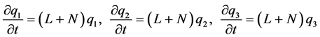 (27)
(27)
where
 (28)
(28)
We solve the system (27) from  to
to  in two splitting steps. We solve first the linear system equation
 (29)
(29)
with the homogenous Dirichlet boundary conditions

using the finite difference method for the time step k, followed by solving the nonlinear system
 (30)
(30)
for the same time step. Equation (30) can be integrated exactly in time [15] , the exact solution is


To apply this method in systematic way, we combine the splitting steps via the standard second order Strang splitting [21] . The flowchart of this method can be des- cribed by the following steps.
Step 1: Solution of the nonlinear problem
 (31)
(31)

Step 2: Solution of the linear problem
The solution of the linear can be obtained using the generalized difference scheme
 (32)
(32)

The solution of this system can be obtained by solving linear block tridiagonal system with constant coefficients using Crouts method, and this can be executed in very efficient way.
Step 3: Solution of the nonlinear problem
 (33)
(33)

The numerical scheme is of second order accuracy in time, second and fourth order in space for  and
and , respectively. It is unconditionally stable and con-
served the conserved quantities exactly [15] [20] [23] . We denote this method by the time splitting finite difference method by (TSFDM).
6. Numerical Results
In this section, we conduct some typical numerical examples to verify the accuracy, conservation laws, computational efficiency and some physical interaction phenomena described by 3-coupled nonlinear Schrödinger equations.
6.1. Single Soliton
In this test, we choose the initial condition as
 (34)
(34)

The following set of parameters are used


The error and the conserved quantities as well as the execution time for all methods are given in Tables 1-6, we have noticed that all method are conserved the conserved quantities exactly and for accuracy the credit goes to the fourth order scheme
 . The profile of
 ,
,  and
and  at different times are displayed in
Figures 1-3. respectively.
To test the convergent rate in space and time of the proposed schemes. We define the  error norm by

where  and
and  are respectively the exact and the numerical solution at the grid

Table 1.Second order scheme (σ = 0) (Algorithm 1), cpu = 2.28 sec.
Table 2.Fourth order scheme (σ = 1/12) (Algorithm 1), cpu = 2.27 sec.
Table 3.Second order scheme (σ = 0) (Algorithm 2), cpu = 3.13 sec.
Table 4.Fourth order scheme (σ = 1/12) (Algorithm 2), cpu = 3.14 sec.
Table 5.TSFDM (σ = 0), cpu = 1.15 sec.
Table 6.TSFDM (σ = 1/12), cpu = 1.41 sec.
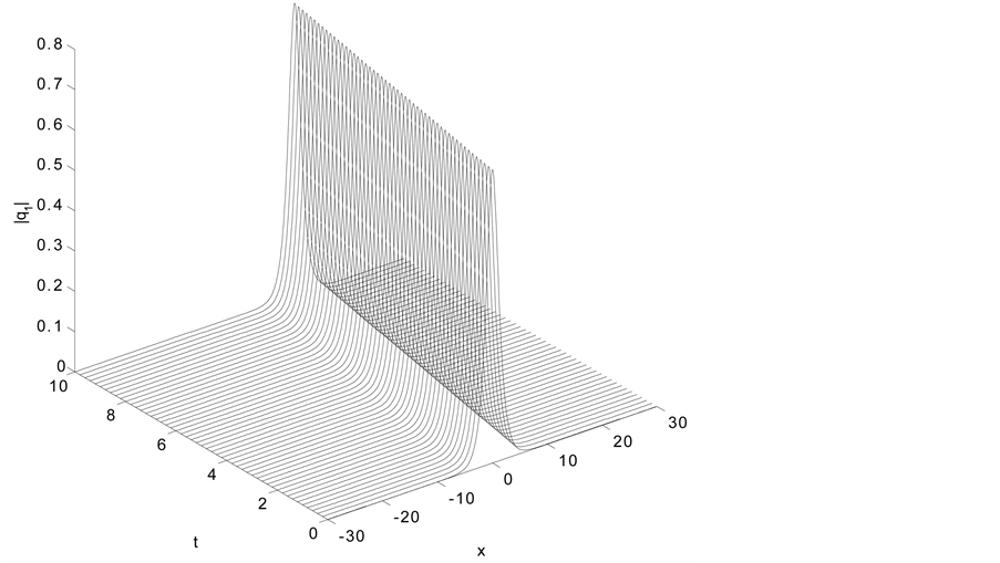
Figure 1. Single soliton: |q1|.
point . In this experiment, we take
 . The convergent rate “order” is calculated by the formula
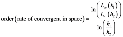
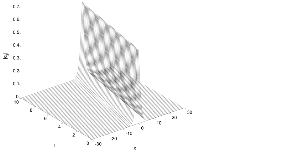
Figure 2. Single soliton: |q2|.

Figure 3. Single soliton: |q3|.
To calculate the convergent rate in space, we take the time step k sufficiently small and the error from temporal truncation is relatively small . From Table 7,
Table 7. Spatial order of convergent with k = 0.0005 at T = 1.
we can easily that the rate of convergent is 4 as we claim in this work.
To check the temporal convergent rate, we fix the spatial step h small enough so that the truncation from space is negligible such as h = 0.01. The results are given in Table 8 which indicate that the order is 2 as we claim in the text.
6.2. Interaction of Two Solitons
To study the interaction of two solitons with different parameters, we choose the initial condition as a sum of two single solitons of the form
 (35)
(35)
where


For all examples in the case of interaction, we choose the set of parameters


together with different values of  for each test. We will study the dynamics of the following cases
Test 1: Two Solitons (with Pure Imaginary Parameters)
In this test we will consider the two set of parameters (equal and different )
 (36)
(36)
and
 (37)
(37)
For the first set of parameters (36), we have noticed that the amplitudes of soliton 1 and soliton 2 before the interaction are  and
and remain unchanged after the interaction which means the interaction is elastic and this scenario is displayed in Figures 4-6.
For the second set of parameters (37), we have noticed that the amplitudes of soliton 1 and soliton 2 before the interaction are  and
and
Table 8. Temporal order of convergent with h = 0.01 at T = 1.

Figure 4. Elastic interaction with equal pure imaginary parameters |q1|.

Figure 5. Elastic interaction with equal pure imaginary parameters |q2|.
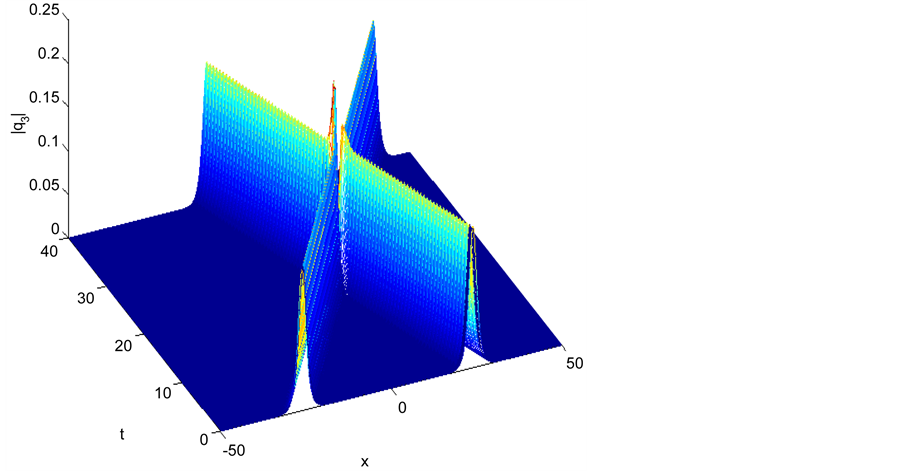
Figure 6. Elastic interaction with equal pure imaginary parameters |q3|.
 change to
  and
and
 after the interaction, the collision mechanism can be described as follows

and in this case we have inelastic collision and we display this scenario in Figures 7-9.
6.3. Test 2: (Pure Real Parameters)
In this test, we choose two different test of parameters
 (38)
(38)
and
 (39)
(39)
For the first set of parameters (38), we have noticed that the amplitudes of soliton 1 and soliton 2 before the interaction are  and
and remain unchanged after the interaction which means the interaction is elastic and this scenario is displayed in Figures 10-12.
For the second set of parameters (39), we have noticed that the amplitudes of soliton 1 and soliton 2 before the interaction are  and
and change to
  and
and after the interaction, this means the collision mechanism is inelastic and can be given as

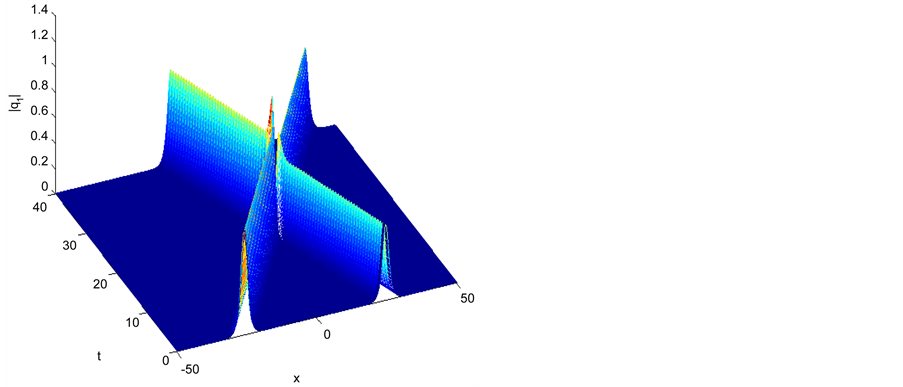
Figure 7. Inelastic interaction with different pure imaginary parameters |q1|.
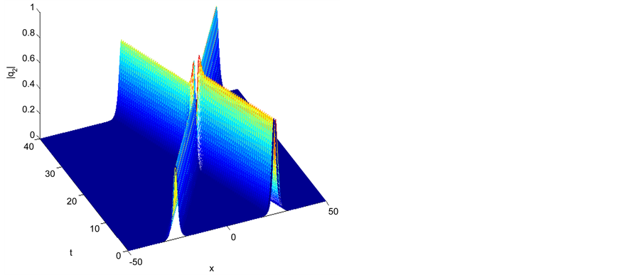
Figure 8. Inelastic interaction with different pure imaginary parameters |q2|.
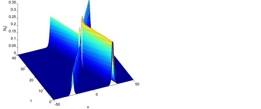
Figure 9. Inelastic interaction with different pure imaginary parameters |q3|.
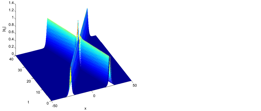
Figure 10. Elastic interaction with pure real parameters q1.

Figure 11. Elastic interaction with pure real parameters q2.

Figure 12. Elastic interaction with pure real parameters q3.

we display the interaction scenario in Figures 13-15.
6.4. Test 3: Soliton Interaction (Nonzero Real and Imaginary Parts)
In this test, we choose the two sets of parameters
 (40)
(40)
and
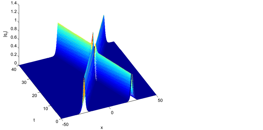
Figure 13. Inelastic interaction with pure real di¤erent parameters q1.

Figure 14. Inelastic interaction with pure real different parameters q2.
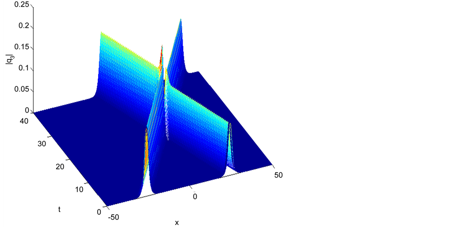
Figure 15. Inelastic interaction with pure real different parameters q3.
 (41)
(41)
For the first set of parameters (40), we have noticed that the amplitudes of soliton 1 and soliton 2 before the interaction are  and
and
 remain unchanged after the interaction which means the interaction is elastic and this scenario is displayed in Figures 16-18.
For the second set of parameters, we have noticed that the amplitudes of soliton 1 and soliton 2 before the interaction are  and
and
 change to
  and
and
 after the interaction, the collision mechanism can be given as follows


and in this case we have inelastic collision and we display this scenario in Figures 19-21.
7. Conclusion
In this work, we have derived different methods for solving the 3-coupled nonlinear Schrödinger equation using finite difference method and time splitting method with finite difference methods. All schemes are unconditionally stable and highly accurate and conserve the conserved quantities exactly. The interaction of two solitons is discussed in details for different parameters. We have noticed that to have elastic interaction the following constraint
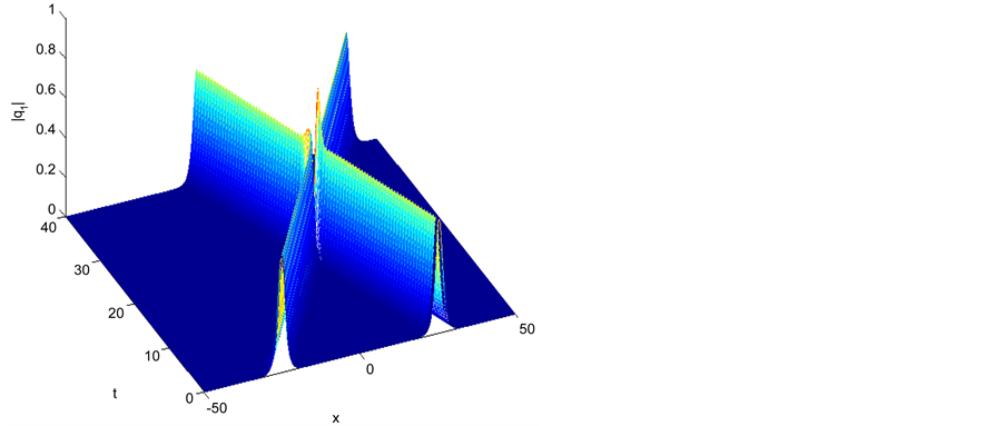
Figure 16. Elastic interaction with non zero real and imaginary parameters for q1.

Figure 17. Elastic interaction with non zero real and imaginary parameters for q2.
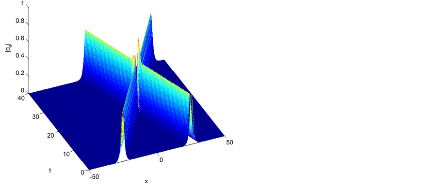
Figure 18. Elastic interaction with non zero real and imaginary parameters for q3.
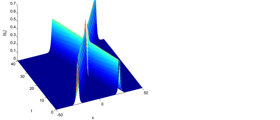
Figure 19. Inelastic interaction with non zero real and imaginary different parameters for q1.
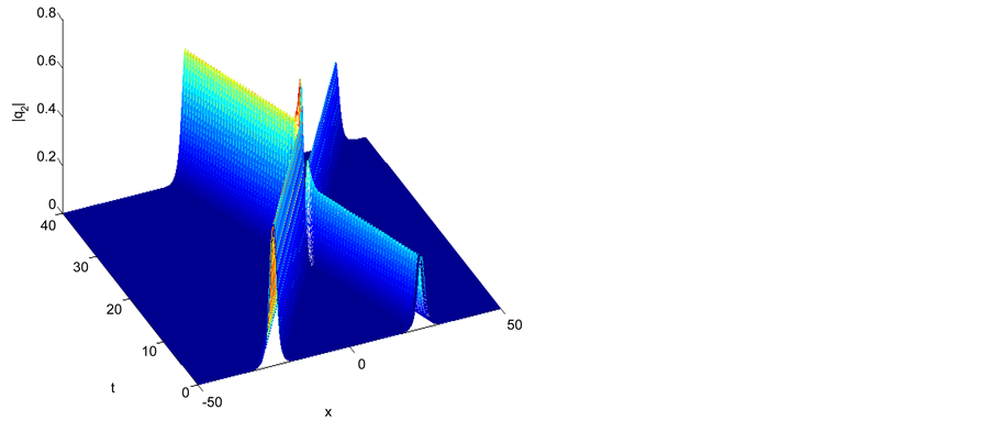
Figure 20. Inelastic interaction with non zero real and imaginary different parameters for q2.
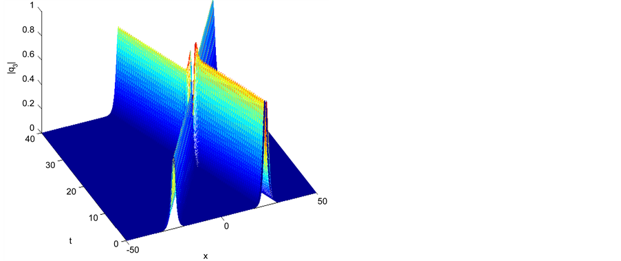
Figure 21. Inelastic interaction with non zero real and imaginary different parameters for q3.

must be satisfied, and for other values the interaction is inelastic, and different behaviors occur (enhancement,suppression) in the amplitude of each soliton. This behavior is in agreement with [1] [2] [3] [4] . The derived methods can be used to solve similar nonlinear problems.
Cite this paper
Ismail, M.S. and Alaseri, S.H. (2016) Computational Methods for Three Coupled Nonlinear Schrödinger Equations. Applied Mathematics, 7, 2110- 2131. http://dx.doi.org/10.4236/am.2016.717168
References
- 1. Kanna, T. and Lakshmanan, M. (2003) Exact Soliton Solutions of Coupled Nonlinear Schrödinger Equation: Shape-Changing Collisions, Logic Gates and Partially Coherent Soliton. Physical Review E, 67, Article ID: 046617.
http://dx.doi.org/10.1103/physreve.67.046617 - 2. Kanna, T. and Lakshmanan, M. (2001) Exact Soliton Solutions, Shape Changing Collisions and Partially Coherent Solitons in Coupled Nonlinear Schrödinger Equations. Physical Review Letter, 86, 5043-5046.
http://dx.doi.org/10.1103/PhysRevLett.86.5043 - 3. Lü, X. and Lin, F. (2016) Soliton Excitations and Shape-Changing Collisions in Alpha Helical Protines with Interspine Coupling at Higher Order. Communications in Nonlinear Science and Numerical Simulation, 32, 241-261.
http://dx.doi.org/10.1016/j.cnsns.2015.08.008 - 4. Lü, X. (2014) Bright-Soliton Collisions with Shape Change by Intensity Redistribution for the Coupled Sasa-Satsuma System in the Optical Fiber Communications. Communications in Nonlinear Science and Numerical Simulation, 19, 3969-3987.
http://dx.doi.org/10.1016/j.cnsns.2014.03.013 - 5. Ismail, M.S. (2008) Numerical Solution of Coupled Nonlinear Schrödinger Equation by Galerkin Method. Mathematics and Computers in Simulation, 78, 532-547.
http://dx.doi.org/10.1016/j.matcom.2007.07.003 - 6. Ismail, M.S., Al-Basyouni, K.S. and Aydin, A. (2015) Conservative Finite Difference Schemes for the Chiral Nonlinear Schrödinger Equation. Boundary Value Problem, 2015, 89.
http://dx.doi.org/10.1186/s13661-015-0350-4 - 7. Ismail, M.S. (2008) A Fourth Order Explicit Schemes for the Coupled Nonlinear Schrödinger Equation. Applied Mathematics and Computation, 196, 273-284.
http://dx.doi.org/10.1016/j.amc.2007.05.059 - 8. Ismail, M.S. and Taha, T.R. (2001) Numerical Simulation of Coupled Nonlinear Schrödinger Equation. Mathematics and Computers in Simulation, 56, 547-562.
http://dx.doi.org/10.1016/S0378-4754(01)00324-X - 9. Ismail, M.S. and Alamri, S.Z. (2004) Highly Accurate Finite Difference Method for Coupled Nonlinear Schrödinger Equation. International Journal of Computer Mathematics, 81, 333-351.
http://dx.doi.org/10.1080/00207160410001661339 - 10. Ismail, M.S. and Taha, T.R. (2007) A Linearly Implicit Conservative Scheme for the Coupled Nonlinear Schrödinger Equation. Mathematics and Computers in Simulation, 74, 302-311.
http://dx.doi.org/10.1016/j.matcom.2006.10.020 - 11. Hu, X. and Zhang, L. (2014) Conservative Compact Difference Schemes for the Coupled Nonlinear Schrödinger System. Numerical Methods for Partial Differential Equations, 30, 749-772.
http://dx.doi.org/10.1002/num.21826 - 12. Kong, L., Ji, L. and Zhu, P. (2015) Compact and Efficient Conservative Schemes for Coupled Nonlinear Schrödinger Equations. Numerical Methods for Partial Differential Equations, 31, 1814-1843.
http://dx.doi.org/10.1002/num.21969 - 13. Bhatt, H.P., Abdul, Q. and Khaliq, M. (2014) Higher Order Exponential Time Differencing Scheme for System of Coupled Nonlinear Schrödinger Equations. Applied Mathematics and Computation, 228, 271-291.
http://dx.doi.org/10.1016/j.amc.2013.11.089 - 14. Xu, Q., Song, S. and Chen, Y. (2014) A Semi-Explicit Multi-Symplectic for a 3-Coupled Nonlinear Schrödinger Equations. Computer Physics Communication, 185, 1255-1264.
http://dx.doi.org/10.1016/j.cpc.2013.12.025 - 15. Antoine, X., Bao, W. and Besse, C. (2013) Computational Methods for the Dynamics of the Nonlinear Schrödinger/Gross-Pitaevskii Equations. Computer Physics Communications, 184, 2621-2633.
http://dx.doi.org/10.1016/j.cpc.2013.07.012 - 16. Aydin, A. and Karasozen, B. (2007) Symplectic and Multisymplectic Methods for Coupled Nonlinear Schrödinger Equations with Periodic Solutions. Computer Physics Communications, 177, 566-583.
http://dx.doi.org/10.1016/j.cpc.2007.05.010 - 17. Bao, W., Tang, Q. and Xu, Z. (2013) Numerical Methods and Comparison for Computing Dark and Bright Solitons in the Nonlinear Schrödinger Equation. Journal of Computational Physics, 235, 423-445.
http://dx.doi.org/10.1016/j.jcp.2012.10.054 - 18. Chen, A., Zhu, H. and Song, S. (2010) Multi-Symplectic Splitting Method for the Coupled Nonlinear Schrödinger Equation. Computer Physics Communications, 181, 1231-1241.
http://dx.doi.org/10.1016/j.cpc.2010.03.009 - 19. Ma, Y., Kong, L. and Cao, Y. (2011) High Order Compact Splitting Multi-Symplectic Method for the Coupled Nonliner Schrödinger Equations. Computers and Mathematics with Applications, 61, 319-333.
http://dx.doi.org/10.1016/j.camwa.2010.11.007 - 20. Talleei, A. and Dehghan, M. (2014) Time-Splitting Pseudo-Spectral Domain Decomposition Method for the Soliton Solutionts of the One-and Multidimensional Nonlinear Schrödinger Equation. Computer Physics Communications, 185, 1515-1528.
http://dx.doi.org/10.1016/j.cpc.2014.01.013 - 21. Wang, S. and Zhang, L. (2011) Split-Step Orthogonal Spline Collocation Methods for Nonlinear Schrödinger Equations in One, Two, and Three Dimensions. Applied Mathematics and Computation, 218, 1903-1916.
http://dx.doi.org/10.1016/j.amc.2011.07.002 - 22. Wang, T., Guo, B. and Zhang, L. (2010) New Conservative Difference Schemes for a Coupled Nonlinear Schrödinger System. Applied Mathematics and Computation, 217, 1604-1619.
http://dx.doi.org/10.1016/j.amc.2009.07.040 - 23. Dehghan, M. and Taleei, A. (2010) A Compact Split Step Finite Difference Method for Solving the Nonlinear Schrödinger Equations with Constant and Variable Coefficients. Computer Physics Communications, 181, 43-51.
http://dx.doi.org/10.1016/j.cpc.2009.08.015