Applied Mathematics
Vol.07 No.14(2016), Article ID:69826,8 pages
10.4236/am.2016.714128
Finite Elements Based on Deslauriers-Dubuc Wavelets for Wave Propagation Problems
Rodrigo Bird Burgos1, Marco Antonio Cetale Santos2
1Department of Structures and Foundations, Rio de Janeiro State University (UERJ), Rio de Janeiro, Brazil
2Department of Geology and Geophysics, Fluminense Federal University (UFF), Niterói, Brazil

Copyright © 2016 by authors and Scientific Research Publishing Inc.
This work is licensed under the Creative Commons Attribution International License (CC BY).
http://creativecommons.org/licenses/by/4.0/


Received 9 June 2016; accepted 14 August 2016; published 17 August 2016
ABSTRACT
This paper presents the formulation of finite elements based on Deslauriers-Dubuc interpolating scaling functions, also known as Interpolets, for their use in wave propagation modeling. Unlike other wavelet families like Daubechies, Interpolets possess rational filter coefficients, are smooth, symmetric and therefore more suitable for use in numerical methods. Expressions for stiffness and mass matrices are developed based on connection coefficients, which are inner products of basis functions and their derivatives. An example in 1-D was formulated using Central Difference and Newmark schemes for time differentiation. Encouraging results were obtained even for large time steps. Results obtained in 2-D are compared with the standard Finite Difference Method for validation.
Keywords:
Wavelets, Interpolets, Deslauriers-Dubuc, Wavelet Finite Element Method, Wave Propagation

1. Introduction
Among the numerous techniques available for the solution of partial differential equations (like the one that describes wave propagation phenomena), the Finite Difference Method (FDM) [1] is by far the most employed one, being used frequently as a standard for the validation of new methods, especially in geophysical applications. As a disadvantage, the FDM is known for requiring excessive refining of the model discretization. Irregular grids can be used, increasing the complexity of the implementation and its computational cost.
The Finite Element Method (FEM) is a versatile tool for solving numerical problems. Its main advantage over other methods is its geometrical flexibility, which allows the use of complex and irregular meshes. Another known advantage of the FEM is how it naturally deals with boundary conditions. Its application to wave propagation problems is still limited, due to the large number of frequencies that are excited in the system [2] . This work proposes adaptations in the FEM which can improve its performance in wave propagation problems.
The conventional formulation of the FEM uses polynomials for interpolating the displacement within the elements (shape functions). This work proposes the use of shape functions based on wavelet scaling functions in order to obtain satisfactory results with less refined meshes and bigger time steps than the traditional FEM and FDM would require without affecting stability and convergence.
Wavelets functions have several properties that are quite useful for representing solutions of partial differential equations (PDEs), such as orthogonality, compact support and exact representation of polynomials of a certain degree. These characteristics allow the efficient and stable calculation of functions with high gradients or singularities at different levels of resolution [3] .
A complete basis of wavelets can be generated through dilation and translation of a mother scaling function. Although many applications use only the wavelet filter coefficients of the multiresolution analysis, there are some which explicitly require the values of the basis functions and their derivatives, such as the Wavelet Finite Element Method (WFEM) [4] - [8] . Compactly supported wavelets have a finite number of derivatives which can be highly oscillatory. This makes the numerical evaluation of integrals of their inner products difficult and unstable. Those integrals are called connection coefficients and they appear naturally in a Finite Element scheme. Due to some properties of wavelet functions, these coefficients can be obtained by solving an eigenvalue problem using filter coefficients and a normalization rule.
Working with dyadically refined grids, Deslauriers and Dubuc [9] obtained a new family of wavelets with interpolating properties, later called Interpolets. Their filter coefficients are obtained from an autocorrelation of the Daubechies’ coefficients. As a consequence, interpolets are symmetric, which is especially interesting in numerical analysis. The use of interpolets instead of Daubechies’ wavelets considerably improves the elements accuracy [10] .
The formulation of an Interpolet-based finite element system is demonstrated for a one-dimensional wave propagation problem. Newmark’s algorithm for direct integration was tried as an alternative to the Central Difference Method in order to allow bigger time steps. A homogeneous example was formulated in order to validate the approach in two-dimensional applications.
2. Interpolating Scaling Functions
Multi-resolution analysis using orthogonal, compactly supported wavelets has become increasingly popular in numerical simulation. Wavelets are localized in space, which allows the analysis of local variations of the problem at various levels of resolution.
All the mathematical foundation for wavelet functions is based on the algorithms for Daubechies wavelets [11] . Wavelet basis are composed of two kinds of functions: scaling functions (φ) and wavelet functions (ψ). The two combined form a complete Hilbert space of square integrable functions. The spaces generated by scaling and wavelet functions are complementary and both are based on the same mother function. In the following expressions, known as the two-scale relation, ak are the scaling function filter coefficients and N is the Daubechies wavelet order:
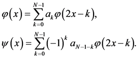 (1)
(1)
The term interpolet was first used by Donoho [12] to designate wavelets with interpolating characteristics. The basic characteristics of interpolating wavelets require that the mother scaling function satisfies the following condition [13] :
 . (2)
. (2)
Any function f(x) can be represented as a linear combination of the basis functions at level of resolution j:
 (3)
(3)
Evaluating the function at a dyadic grid point x = 2−jr yields:
 . (4)
. (4)
This characteristic is very interesting for numerical applications, since a function can be represented as a weighted sum in which the coefficients are evaluations of the same function at target points on a dyadic mesh:
 . (5)
. (5)
The Deslauriers-Dubuc interpolating function of order N is given by an autocorrelation of the Daubechies’ scaling filter coefficients (hm) of the same order (i.e. N/2 vanishing moments, given in [11] ). Its support is given by [1 − N N − 1], it has even symmetry and is capable of representing polynomials of order up to N − 1. Interpolets satisfy the same requirements as other wavelets, especially the two-scale relation (using a support adjustment):
 (6)
(6)
Table 1 shows the typical values of filter coefficients for interpolets of orders 4, 6 and 8.
Figure 1 shows the interpolet IN6 (autocorrelation of DB6). Its symmetry and interpolating properties are

Table 1. Filter coefficients for Deslauriers-Dubuc interpolets (ak = a−k).

Figure 1. Interpolet IN6 scaling function.
evident. It is capable of representing a 5-degree polynomial. Its Daubechies “mother” of same order would only represent a 2-degree polynomial.
3. Wave Propagation
The partial differential equation (PDE) which rules the wave propagation is:
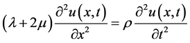 , (7)
, (7)
where, u is the horizontal displacement, ρ is the density, t is the time and λ and μ are the Lamé parameters of the medium. Applying Hamilton’s Principle and using the FEM, the PDE can be rewritten at a specific time t as a system of linear equations, which in matrix form is:
 . (8)
. (8)
In the given expression, M represents the mass matrix and K is the stiffness matrix of the model. These FEM system global matrices are assembled from the individual contributions of the local matrices of each element.
As in the FDM, it becomes necessary to solve the system of equations at discrete time intervals. There are several effective direct integration methods, among which the most intuitive one is the Central Difference Method, given by:
 . (9)
. (9)
Substituting the expression of the acceleration obtained by the Central Difference Method and solving for the next time step t+Δtu gives:
 . (10)
The result of the matrix operation M−1K is obtained directly if M is diagonal. In this case, one can generate a unique local matrix at element level which contains both mass and stiffness information. It is known that the diagonal mass matrix can be used instead of the one generated from shape functions (consistent matrix) without introducing significant errors in the system. Nevertheless, in this work consistent mass matrices were used and a global matrix X was assembled using mass and stiffness contributions to the system. Stability of the Central Difference Method is conditioned to the choice of the time step, whose upper bound is obtained from a generalized eigenvalue problem.
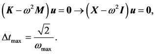 (11)
(11)
3.1. Newmark Method
The constant-average-acceleration method (a special case of the Newmark Method) consists in an unconditionally stable scheme which can be summarized by the following expression (as given in [2] ):
 . (12)
This method requires the calculation of velocity and acceleration at all time steps and the inversion of the left hand side operator. Despite this, the Newmark Method is unconditionally stable. Therefore, significantly bigger time steps can be used.
3.2. Application to 2-D Problems
The PDE for the 2-D axial displacement wave equation is:
 , (13)
which can still be solved using 1-D finite elements by applying a scheme similar to what is commonly done in the FDM:
 . (14)
In the expression above, a second stiffness matrix is introduced as a differential operator in the second space dimension. The displacement is also represented as a matrix, instead of the usual vector representation of the FEM. Matrices X e ZT perform the differentiation along x and z directions respectively. These matrices contain both mass and stiffness information. Assuming spatial sampling of Nx × Nz points, X and Z are of size Nx × Nx and Nz × Nz, respectively. This represents an improvement over traditional FEM in terms of computational effort; usually, the FEM requires a displacement vector of length Nx × Nz and both global stiffness and mass matrices must have a size of (Nx × Nz) ×(Nx × Nz), operating over the whole system.
The application of the Newmark Method in this 2-D scheme is not as simple as in 1-D, since the elements are still one-dimensional and there are right and left matrix multiplications involved. The following expression is an adaptation of the Newmark Method to the 2-D implementation proposed:
 . (15)
In this expression, t+Δtu appears in both sides of the equation, thus requiring the application of an iterative method for its calculation. This procedure not only increases the computational effort significantly but can also cause instability for large time steps.
4. Finite Element Formulation
Assuming that displacement u is approximated by a series of interpolating scale functions, the following may be written:
 . (16)
Stiffness and mass matrices can be obtained by solving the wave propagation PDE using the FEM. Dimensionless coordinates (ξ) within the interval [0 1] are used in wavelet space, which leads to the subsequent expressions:
 (17)
(17)
The so-called connection coefficients Γ appear in the expressions above. Wavelet dilation and translation properties allow the calculation of connection coefficients to be summarized by the solution of an eigenvalue problem based only on filter coefficients [14] .
 (18)
(18)
Since the expression above leads to an infinite number of solutions, there is the need for a normalization rule that provides a unique eigenvector. This unique solution comes with the inclusion of the so-called moment equation, derived from the wavelet property of exact polynomial representation, which is given originally in [15] and adapted for Interpolets by [8] :
 (19)
(19)
The dimensionless expressions for the stiffness  and mass
  matrices are in wavelet space and need to be transformed to physical space, using a transformation matrix T obtained by evaluating the wavelet basis at the element node coordinates using Equation (16). It can be noticed that some terms related to the length (L) of the element emerge from coordinate changes.
 (20)
(20)
5. Examples
To validate the formulation of the interpolet-based finite element, a 1-D example was tested. It consists in applying a forced displacement at the free end of a pinned, unit length rod (Figure 2). The propagation was modeled by the FDM using 601 points and Δt = 0.1 ms. For the FEM based on the IN6 interpolet, the discretization was performed with 91 points and Δt = 1 ms. The rod’s middle point time response for both methods is shown in Figure 3, which shows that the FEM result is acceptably close to that of the FDM, especially considering that FEM generates over 60 times less data per simulated second.
In order to validate the 2-D formulation, a simple example was proposed by analyzing the propagation in a 2 km × 2 km model with a constant velocity of 3000 m/s. Finite Element model was sampled every 6.17 m in both directions with a time step Δt of 0.46 ms, obtained by the generalized eigenvalue problem already described. Non-integer values appear due to the 11 degrees-of-freedom present in the element implemented with IN6. A Newmark scheme was also implemented using the same spatial sampling and Δt = 0.6 ms. The results were compared to the FDM using 5 m spacing in both directions and Δt = 0.2 ms. Finite Element mesh has 325 × 325 points and Finite Difference mesh has 401 × 401. Results are shown in Figure 4. Even with a less refined mesh and a more than twice bigger time step, the IN6 element was able to identify characteristic peaks of the wave propagation. The results of the proposed adaptation to the Newmark Method were very similar to the Central Difference ones using an even bigger time step.
6. Conclusions
This work presented the formulation and validation of an interpolet-based finite element. Newmark’s method for time discretization appears promising, although its application in 2-D problems with 1-D elements remains a challenge. The main improvement in the presented formulation was the possibility of using a bigger time step

Figure 2. Unit length rod under forced displacement.

Figure 3. FEM results using IN6 interpolet and newmark method (Δt = 1 ms) compared to FDM (Δt = 0.1 ms) for a one-dimensional wave propagation.

 (a) (b)
 (c) (d)
Figure 4. Propagation snapshots at time t = 0.3 s for 2-D example using: (a) FEM and Central Difference Method, (b) FEM and Newmark Method, (c) FDM and Central Difference Method; (d) comparison of amplitudes along the indicated segment at depth 1000 m.
than the one required by the FDM. In future works, models with greater complexity will be analyzed and different families of wavelets will be explored.
The number of DOFs present in interpolets leads to non-dyadic divisions within the element, requiring an additional approximation which introduces errors in the transformation matrix. The inaccuracy in some values can be attributed mostly to these approximation errors.
As done in the traditional FEM, all matrices involved can be stored and operated in a sparse form, since most of their components are null, thus saving computer resources.
Acknowledgements
Authors would like to thank CNPq and FAPERJ for their financial support.
Cite this paper
Rodrigo Bird Burgos,Marco Antonio Cetale Santos, (2016) Finite Elements Based on Deslauriers-Dubuc Wavelets for Wave Propagation Problems. Applied Mathematics,07,1490-1497. doi: 10.4236/am.2016.714128
References
- 1. Kelly, K.R., Ward, R.W., Treitel, S. and Alford, R.M. (1976) Synthetic Seismograms: A Finite-Difference Approach. Geophysics, 41, 2-27.
http://dx.doi.org/10.1190/1.1440605 - 2. Bathe, K.J. and Wilson, E.L. (1976) Numerical Methods in Finite Element Analysis. Prentice Hall, Upper Saddle River.
- 3. Qian, S and Weiss, J. (1992) Wavelets and the Numerical Solution of Partial Differential Equations. Journal of Computational Physics, 106, 155-175.
http://dx.doi.org/10.1006/jcph.1993.1100 - 4. Ma, J., Xue, J., Yang, S., He, Z. (2003) A Study of the Construction and Application of a Daubechies Wavelet-Based Beam Element. Finite Elements in Analysis and Design, 39, 965-975.
http://dx.doi.org/10.1016/S0168-874X(02)00141-5 - 5. Chen, X., Yang, S., Ma, J. and He, Z. (2004) The Construction of Wavelet Finite Element and Its Application. Finite Elements in Analysis and Design, 40, 541-554.
http://dx.doi.org/10.1016/S0168-874X(03)00077-5 - 6. Han, J.G., Ren, W.X. and Huang, Y. (2005) A Multivariable Wavelet-Based Finite Element Method and Its Application to Thick Plates. Finite Elements in Analysis and Design, 41, 821-833.
http://dx.doi.org/10.1016/j.finel.2004.11.001 - 7. He, Y., Chen, X., Xiang, J. and He, Z. (2008) Multiresolution Analysis for Finite Element Method Using Interpolating Wavelet and Lifting Scheme. Communications in Numerical Methods in Engineering, 24, 1045-1066.
http://dx.doi.org/10.1002/cnm.1011 - 8. Burgos, R.B., Cetale Santos, M.A. and Silva, R.R. (2013) Deslauriers-Dubuc Interpolating Wavelet Beam Finite Element. Finite Elements in Analysis and Design, 75, 71-77.
http://dx.doi.org/10.1016/j.finel.2013.07.004 - 9. Deslauriers, G. and Dubuc, S. (1989) Symmetric Iterative Interpolation Processes. Constructive Approximation, 5, 49-68.
http://dx.doi.org/10.1007/BF01889598 - 10. Burgos, R.B., Cetale Santos, M.A. and Silva, R.R. (2015) Analysis of Beams and Thin Plates Using the Wavelet-Galerkin Method. International Journal of Engineering and Technology (IJET), 7, 261-266.
http://dx.doi.org/10.7763/IJET.2015.V7.802 - 11. Daubechies, I. (1988) Orthonormal Bases of Compactly Supported Wavelets. Communications in Pure and Applied Mathematics, 41, 909-996.
http://dx.doi.org/10.1002/cpa.3160410705 - 12. Donoho, L.D. (1992) Interpolating Wavelet Transforms.
http://statweb.stanford.edu/~donoho/Reports/1992/interpol.pdf - 13. Shi, Z., Kouri, D.J., Wei, G.W. and Hoffman, D.K. (1999) Generalized Symmetric Interpolating Wavelets. Computer Physics Communications, 119, 194-218.
http://dx.doi.org/10.1016/S0010-4655(99)00185-X - 14. Zhou, X. and Zhang, W. (1998) The Evaluation of Connection Coefficients on an Interval. Communications in Nonlinear Science & Numerical Simulation, 3, 252-255.
http://dx.doi.org/10.1016/S1007-5704(98)90044-2 - 15. Latto, A., Resnikoff, H.L. and Tenenbaum, E. (1992) The Evaluation of Connection Coefficients of Compactly Supported Wavelets. In: Maday, Y., Ed., Proceedings of the French-USA Workshop on Wavelets and Turbulence, Princeton University, June 1991, Springer-Verlag, New York, 76-89.