Applied Mathematics
Vol.05 No.18(2014), Article ID:51047,14 pages
10.4236/am.2014.518273
Automated Cell Detection and Morphometry on Growth Plate Images of Mouse Bone
Maria-Grazia Ascenzi1*, Xia Du1, James I. Harding1, Emily N. Beylerian2, Brian M. de Silva2, Ben J. Gross2, Hannah K. Kastein2, Weiguang Wang1, Karen M. Lyons1, Hayden Schaeffer3
1Department of Orthopaedic Surgery, University of California, Los Angeles, California, USA
2Department of Mathematics, University of California, Los Angeles, California, USA
3Department of Mathematics, University of California, Irvine, California, USA
Email: *mgascenzi@mednet.ucla.edu
Copyright © 2014 by authors and Scientific Research Publishing Inc.
This work is licensed under the Creative Commons Attribution International License (CC BY).
http://creativecommons.org/licenses/by/4.0/


Received 17 August 2014; revised 23 August 2014; accepted 11 September 2014
ABSTRACT
Microscopy imaging of mouse growth plates is extensively used in biology to understand the effect of specific molecules on various stages of normal bone development and on bone disease. Until now, such image analysis has been conducted by manual detection. In fact, when existing automated detection techniques were applied, morphological variations across the growth plate and heterogeneity of image background color, including the faint presence of cells (chondrocytes) located deeper in tissue away from the image’s plane of focus, and lack of cell-specific features, interfered with identification of cells. We propose the first method of automated detection and morphometry applicable to images of cells in the growth plate of long bone. Through ad hoc sequential application of the Retinex method, anisotropic diffusion and thresholding, our new cell detection algorithm (CDA) addresses these challenges on bright-field microscopy images of mouse growth plates. Five parameters, chosen by the user in respect of image characteristics, regulate our CDA. Our results demonstrate effectiveness of the proposed numerical method relative to manual methods. Our CDA confirms previously established results regarding chondrocytes’ number, area, orientation, height and shape of normal growth plates. Our CDA also confirms differences previously found between the genetic mutated mouse Smad1/5CKO and its control mouse on fluorescence images. The CDA aims to aid biomedical research by increasing efficiency and consistency of data collection regarding arrangement and characteristics of chondrocytes. Our results suggest that automated extraction of data from microscopy imaging of growth plates can assist in unlocking information on normal and pathological development, key to the underlying biological mechanisms of bone growth.
Keywords:
Anisotropic Diffusion, Cell Detection, Growth Plate, Mouse, Retinex

1. Introduction
Microscopy imaging of mouse growth plates is extensively used to assess development and potential pathology. Such imaging confounds current automated methods for cell detection. Indeed, application to microscopy images of growth plates of each of the classic methods of image segmentation and processing (e.g. Canny segmentation [1] , cartoon-texture decomposition [2] , k-means clustering [3] ) does not take into account that: 1) the color intensity of each stain used to visualize a specific biological component can vary throughout the growth plate; 2) the characteristics (e.g. size, shape, orientation) of cells (chondrocytes) vary greatly within healthy, normal growth plate; and 3) the shades of colors within cells are present outside cells. Moreover, the cells (chondrocytes) positioned beneath the plane of focus of the image appear faintly, yielding a highly non-homogeneous background to the cells on the plane of focus. Current cell detection algorithms apply to simpler images that show either a more homogeneous background or the presence of a cell-specific characteristic (e.g. intensity or nucleus) usable as a starting point for cell detection [4] -[9] .
Analysis of chondrocytes’ number, size, orientation, height and shape offer insights on the developmental effects of repressing various genes, the lack of which can lead to bone growth disorders (e.g. [10] [11] ). Longitudinal growth of bones is the result of a process involving cell division, migration, and then ossification that occurs in growth plates located at both the proximal and distal ends of the long bone. In healthy growth plates, the chondrocytes sequentially differentiate into four sub-types, including resting, proliferating, prehypertrophic and hypertrophic chondrocytes, stratified from each end of the bone towards its center (for reviews, [12] [13] ). Throughout the growth plate, only some nuclei are visible with appropriate stain. The resting zone contains relatively quiescent small, round, densely packed cells. Upon entry in the proliferating zone, cells elongate medial-laterally and undergo division by mitosis. At each division, the newly produced daughter cell remains closely situated with respect to the mother cell but may be far apart from other cells. The cells begin to form stacks. In pre-hypertrophic and hypertrophic zones, chondrocytes become arranged in columns. Such cells begin to enlarge and express Indian Hedgehog while the expression of Sox9 is reduced [14] . In the hypertrophic zone, the terminal enlarged chondrocytes are larger than that in the rest of the growth plate, either round or elongated in the longitudinal direction, and packed closely to one another. The bottom of this region is marked by ossification [15] , [16] . Correlations exist among height of hypertrophic chondrocytes, growth plate length, and limb length [17] .
In this paper, we propose a method of automated multi-step image processing. These steps prepare an image for automated measurement of the characteristics of the chondrocytes located on the plane of focus of the original growth plate specimen. Rather than manually determining cell profiles, automated cell detection, and subsequent automated morphometry would aid biological research by increasing efficiency of measurements.
2. Methods
2.1. Microscopy
The ideal image should be of a specimen whose preparation involves a stain that maximizes the contrast between cell cytoplasm and background, and in focus throughout. We visualized chondrocytes in the growth plate of mice ex vivo with a BX60 microscope (Olympus America) set to bright-field. The animal protocol was approved by UCLA’s Animal Research Committee. Male mice on mixed background, predominantly 129/SvJ crossed with C57Bl6/J (WT for wild type), were sacrificed at perinatal 0, two weeks, four months. After isolation of hind limbs, we stained coronal sections of femora and tibiae to visualize cartilage (with Alcian blue or Safranin O), cell cytoplasm (Fast Green) and nucleus (Hematoxylin) [18] [19] . We took TIFF images of sections at 60× and 100× magnification.
2.2. Image Preparation
We imported the TIFF images of growth plates into software XaraX version 1.1 (XaraX Group). The Shape Editor, Combine Shapes and Intersect Shapes allow tracing of the region of interest (ROI), cropping along the traced line to eliminate the image of the tissue surrounding the growth plate and possibly select a region of the growth plate, and replacement with a white background (Figure 1). This step is necessary to avoid interference of colors that do not belong to the ROI during algorithm application. We then exported the cropped image as TIFF image with same resolution as the original image.
2.3. Cell Detection Algorithm (CDA)
Our CDA is written with and runs on MATLAB version R2012a (Math Works), and is available for download as file CDAlg.m together with three of the full resolution images on which the CDA was run to prepare some of the figures in this paper, from https://sites.google.com/site/bthsca/automated-cell-detection-1. The input for the CDA consists of a TIFF image (Figure 1). The output is a black and white (i.e. binary) image of the size of the input image, with white pixels representing cells on a black background. The CDA consists of 5 steps:
Step 1: We assign similar intensity values to cells in focus while we render the background, defined as cells out of focus and extracellular matrix, more homogeneous. We use the color blending method of Retinex, originally developed to simulate the visual cortex blending of colors [20] [21] , and then widely applied to imaging [22] [23] . We use the formalization of Retinex in terms of a Poisson equation [24] . Given an initial image, f, we seek a reconstructed image u with
 (1)
(1)
where
 (2)
(2)
is the discrete Laplacian at pixel, (i, j) and
 (3)
(3)
where
 (4)
(4)

Figure 1. Image of two-week old WT growth plate viewed with bright-field microscopy after excluding surrounding tissue (inset). Cytoplasm is stained gray-green with Fast Green; nuclei are black with Hematoxylin; cartilage, mucin and mast cell granules are pink-red with Safranin O; and bone is blue with Fast Green.
is the hard thresholding function and τ the thresholding parameter. Thus, if a small gradient (of magnitude smaller than τ) is present at a pixel, it is replaced with zero. The Poisson equation then constructs the image whose gradient most closely matches the vector field that models the difference between each pixel and its neighboring pixels. We use the following semi-implicit scheme that converges rapidly to the steady state for local variations:
 (5)
(5)
We apply this process iteratively, NI (number of iterations) times, each time to the previous resultant image.
Step 2: We enhance cell profiles (edges) with anisotropic diffusion. The anisotropic diffusion function needs to discriminate intensity changes by location: near vs. far from edges, and along vs. across edges [25] . Let f be an image, u the filtered image and D the diffusivity tensor. We used the numeric approximation
 (6)
(6)
for single time-steps  (5.3 of [26] ) to solve
 (7)
(7)
with g and 1 set as eigenvalues of D.
Step 3: We extract cell profile information with gradient thresholding. We use the gradient matrix generated in Step 2, containing values scaled between 0 and 255. The hard threshold parameter, called S for “separation”, is chosen to identify single cells within packed clusters, while minimizing pixel loss from cell profile. We use the same Equation (4) with S replacing τ. We obtain a binary representation of the image with white cell profiles on black background suitable for subsequent morphometric analysis.
Step 4: We use the convex hull operation [27] to identify the smallest convex set of points that fully encloses the profile of each cell. This operation renders the profile connected and filled because the thresholding needed to obtain the binary representation at Step 3 may have caused interruptions of the cell profile. This operation is appropriate because 1) cells show an elliptical and therefore convex shape [28] ; and 2) the number of missing pixels from the profile, minimized in Step 3, is small. However, when two cells in focus are close to each other, the two separate cells may lump together and their profiles may form a larger concave shape.
Step 5: We eliminate profiles that do not reflect actual cell size or shape with hard tresholding. Overly large or overly small or misshaped profiles are often created during convexification because of proximity of incomplete profiles or proximity of an incomplete profile with the boundary of the growth plate region. Alo (area lower) and Aup (area upper) bound in pix2 define a range out of which the profiles are excluded. Because these boundaries depend on image size and magnification, they need to be set by the user. Further, we use set up shape thresholding in terms of isoperimetric ratio (IR)
 (8)
(8)
where A denotes area and P perimeter of the shape. The threshold was set at 0.5 because an NI greater than 0.5 demonstrate geometriesS different from ellipses.
The proposed CDA, implemented with MATLAB R2012a with 64-bit Windows-7, an Intel@CoreTM i3-370M processor (2.40 GHz) and 4 GB of RAM, takes between  and
and  sec/pix to create the output image with memory usage of 0.000149 mb/pix (Appendix 1). The computational cost O(MN) of running the CDA on an M × N image is at most equal to HMN for some finite constant H, as M and N approach infinity (Equation (9) of Appendix 2).
2.4. Manual Cell Detection (MCD)
MCD was conducted on 390 cells on a total of three images with XaraX software, for comparison with the CDA. Because chondrocytic two-dimensional profiles throughout the growth plate are best modeled as ellipses [28] , we used Ellipse and Rotation tools to fit a white ellipse to each cell profile that appeared in focus. Because we traced only cells in focus, there is no issue of tracing cells that appear to overlap. By drawing a black background as large as the original image, we obtained a black and white image that was exported at the original image resolution.
2.5. Automated Morphometry of Images
We conducted morphometry on images from each of CDA and MCD with MetaMorph software (Molecular Devices). The Color Threshold was set from 127 to 255 for each of Red, Green and Blue. We calibrated MetaMorph in conjunction with the magnification used to generate the image to measure lengths in real microns. The output parameters were cell number, area, orientation (measured with respect to the long bone axis, counterclockwise from −90˚ to 90˚), height, and shape in terms of isoperimetric ratio IR (see Equation (8)).
2.6. Statistical Analysis
The robustness of the morphometric MCD was measured in terms of inter- and intra-observer errors. The magnitude of these errors was assessed for cell number, area, orientation, height and IR. To assess the magnitude of such errors, the cell profile of six randomly chosen cells in focus was manually drawn with XaraX and measured with MetaMorph forty-two times by each of two observers, twice, two months apart. Further, to detect significant differences between CDA and MCD, and between adjacent zones of a given image, we used the t-test for each of the measured parameters, and the Dice index to measure similarity of cell shapes [29] [30] . Because the sample size is greater than 40, the possible skewness of the data distribution does not affect the robustness of the t-test. We consider a p-value smaller than 0.05 as statistically significant. The collected data are presented as mean ± standard deviation.
3. Results
We have developed an automated method for analysis of growth plate images. Figure 2 shows intermediate images and output image of the CDA.
3.1. CDA
The CDA depends on the five parameters τ, NI, S, Alo, and Aup whose values depend on the image characteristics: τ (Step 1, Equation (4)) is the threshold value at which small visual differences between a given pixel and its neighborhood are eliminated. At small values, we obtain numerous white dots corresponding to either miscellaneous background details or cell fragments. At high values, all cells are homogenized into the background and therefore not detected. NI, the number of iterations of Step 1, has an upper bound, beyond which the cell profiles become too blurry for correct detection. When NI is appropriately smaller than such upper bound, it sufficiently homogenizes the background noise without blurring the cell profile. S is used to identify the cell profile (Step 3). S has an upper bound below which it identifies cell profiles with small pixel gradients. The use of small pixel gradients has the benefit of identifying the complete cell, at the expense of multiple cell aggregation. Higher values of S tend to identify only the high contrast between the nucleus and the stained background leading to reduced cell aggregation, but also to partial cell detection. For stains that do not provide good contrast between cell on plane of focus and background, a low value for S is necessary to detect the small pixel gradients defining the cell profiles. For stains that provide high contrast between the majority of the cells in focus and background, a higher value of S is suitable. Alo and Aup (Step 5) control the area of the detected shape: Alo eliminates leftover minute fragments and Aup eliminates oversize shapes that cannot represent cells.
With appropriate values of the parameters, the CDA analysis confirmed known facts regarding the mouse growth plate in tibia and femur [16] [31] . For the WT, the mean cell area is significantly smaller in the resting zone than in the proliferative zone. Table 1 shows data from a femur as mean ± standard deviation. Significant differences are shown between adjacent zones of the growth plate with ^ for p < 0.01 The values of Alo was optimized for the resting zone that contains the smallest cells. The large standard deviations of cell area are due to proliferation that significantly increases cell size and to hypertrophy that further increases cell size. The significant differences in mean cell area among zones results from distributions of resting, proliferative and hypertrofic cell areas with tails that become significantly longer as cell size increases from resting to hypertrophic zone. This is also the reason why cell area from the three zones ranges shows only a small partial overlap, and give rise to significant differences in cell areas between adjacent zones.
The CDA captures more cell area (per cell) in the proliferative zone because it picks up the parts of the cell which are stained: the CDA is far more sensitive to small gradients in color change, hence it is better able to pick up the color transition between the background and cytoplasm even if the stain bleeds into the cell. We
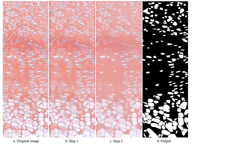
Figure 2. Input, intermediate steps and output of the CDA obtained with 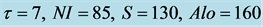 and
and . (a) Original image, detail of Figure 1; (b) Image resulting from reduction of visibility of cells out of focus, and of inconsistencies in background shading and luminosity (Step 1); (c) Cartoon-like component image resulting from application of low diffusion across edges and high diffusion at locations of noise and small features (Step 2); (d) Output image resulting from gradient thresholding to address cell separation (Step 3), convexification (Step 4), and size and shape thresholding (Step 5). Cell clustering can be reduced or eliminated by choosing zone-specific values for and S (see Figure 4).

Table 1. Data from femoral section stained with Alcian Blue and Hematoxylin for , NI = 85, S = 130, Alo = 80, Aup = 20,000.
found that the mean cell area is significantly smaller in the proliferative zone than in the hypertrophic zone; and that the mean orientation differs significantly between resting and proliferative, but not between proliferative and hypertrophic zones. Further, the mean isoperimetric ratio IR is significantly different between resting and proliferative zones, and between proliferative and hypertrophic zones, indicating that the cells become less circular as they progress from the resting to proliferative, and from proliferative to hypertrophic zone. Furthermore, our CDA confirms the rounder shape, and the orientation off the horizontal (medial-lateral) direction, of chondrocytes in the Smad1/5CKO mutant in comparison with the control WT mouse (Figure 3), previously determined by manual detection [10] . Note that for the CDA analysis of this WT growth plate, the Retinex parameter NI was set to zero because these fluorescent microscopy images showed no faint cells behind the plane of focus. In fact, Retinex color blending on inherently high contrast fluorescent microscopy images would reduce the contrast between cell profile and background, making cell detection sub-optimal.

Figure 3. Genetic mutation Smad1/5CKO vs. control mouse. The chondrocytes on the plane of focus of these fluorescent images (a, b) are detected with c)  and
and ; and d) with
  and
and . Orientations are marked in (e, f) to emphasize differences.
3.2. MCD
The 390 cells were chosen on the plane of focus of a total of three images by human eyesight judgment. The chosen cells showed presence of the 92 to 100 range of Red, 62 to 100 of Green and 55 to 100 for Blue. The out-of focus cells appearedoverall darker with 86 to 100 range of Red, 49 to 97 of Green, and 45 to 100 of Blue. The inter- and intra-observer errors for a unique measurement were found to be smaller than 1.5%. We show the data of the calculation of inter- and intra-observer errors concerning the cell area from Figure 1 (Table 2). The minimum (min), maximum (max), mean, and standard deviation (stdev) of distributions of 42 measurements of 6 cell areas provide data for calculation of comparison relative to observer (Obs) 1 and 2 during first (I) and second (II) setting, in terms of % errors (in italics) for measurements considered either paired (p) or unpaired (u) All % errors are smaller than 1.5%. The error of a unique measurement is at most equal to either the difference of the two largest measurements divided by the smallest measurement, if the measurements of the two sets are considered paired (comparison of two measurements of the same cell), or to the largest measurements’ difference divided by the smallest length, if the measurements of the two sets are considered unpaired. On the basis of the small magnitude of the above-analyzed morphometric errors, performance of one measurement by a single observer was deemed appropriate. The computation of errors on six cells per image remained smaller than 1.5%.
3.3. Comparison between CDA and MCD
The best detection of the CDA in comparison to MCD occurs with a 5% difference on 390 cells detected on three images, a Dice similarity index of 0.88 in cell number, and no significant differences for cell position, area, orientation, height, shape factor in terms of isoperimetric ratio. In particular, this means that the convexification step in the CDA did not produce a shape with significant distortion. The aggregation of adjacent cells was present in all zones of the growth plate when single values were assigned to each of τ and S for the whole growth plate. To decrease such aggregation, the parameters τ and S need to vary across the growth plate, specified for each of resting, proliferative and hypertrophic zones, due to variation of relative distance among cells.
Table 2. Assessment of inter- and intra-observer errors.
The hypertrophic zone presents the highest challenge to the CDA because the cells are tightly packed and their profiles frequently touch (Figure 4(a), Figure 4(b)). The analogy of best images for different values of τ and S. (Figures 4(c)-(e)) is indicative of the synergistic effect of τ and S and that the parameters’ values are not 1-to-−1. Within the context of the relation between hypertrophic cell height and length of growth plate, bone and limb ([4] [17] ), we found small variations in hypertrophic cell height and growth plate length to mean hypertrophic cell height ratio (Figures 4(c)-(e); Table 3) for different choices of CDA parameters. In Table 3, the data are presented as mean ± standard deviation. *indicates significant difference in height with , where n = 6 in Bonferroni’s coefficient for multiple comparisons, between pair
  and pair
 , for which the best cell detection occurs (shown in italics). For all runs, NI = 85, Aup = 20,000. Figure 5 shows another example of CDA running with different parameters’ values that focuses on the middle of a primary ossification center (bottom) and of a secondary ossification center (top).
4. Discussion
We have developed a specialized algorithm, implemented in MATLAB, which performs the automated detection of cells in growth plate images. We have used the algorithm to verify known biological characteristics of the mouse growth plate and provide a tool for further research regarding, e.g., implications of height of hypertrophic chondrocytes on limb length.
During the process of developing CDA, we considered current methods for image detection. Canny segmentation, cartoon-texture decomposition (Figures 6(a)-(c); [1] [2] [32] -[34] ) created false positive cell detection from intensity variations of stain. Intensity variations produced also inconsistent clustering of background pixels and cell pixels with k-means clustering (Figure 6(d); [2] [3] ), which clusters data points on similarity basis. Current cell detection algorithms, such as Cell Profiler [4] and HT-HCS [5] , do not apply to our images because they are based on existence of “primary objects” (such as presence of cell-specific intensity), one per cell. We quantitatively compared our CDA to image enhancing processor Image J [6] that includes various filtering, thresholding, segmentation compared our CDA to image enhancing processors Image J [6] that includes various filtering, thresholding, segmentation and clustering methods [7] , with a recent implementation to detect single cells on a slide [8] . We compared each of Image J and CDA  to MCD of 390 cells from three images. We obtained the best readable image with Image J, by first rendering the background more homogeneous with a 50% contrast enhancement. Then to obtain a black and white image, we used color threshold “HSB color space” to threshold black and white. Afterwards, we adjusted hue, saturation and brightness to maximize individual cell detection. We found that Image J picks up background cells out of focus and often separates visible nuclei from cells. Therefore, Image J generates at least a 26% difference in cell count in comparison with the MCD results. This percentage is larger than the 5% difference generated by the CDA with respect to the MCD. Image J showed no significant difference with MCD for cell area, orientation and height while the shape factor (isoparametric ratio) differed significantly between Image J and MCD. This in comparison to no significant differences for cell area, orientation, height and shape factor on all three images obtained with the CDA. Further, any CDA output image can be processed with existent software to assess more complex parameters for object and pattern assessment [35] -[38] .
Recently, Buggenthin et al. [9] developed an algorithm for detection of hematopoietic stem cell in culture on

Figure 4. Specification of parameters  and S for hypertrophic zone of tibia’s growth plate of neonatal (P0) WT mouse. (a) This is the original image of growth plate where the cartilage is stained with Alcian blue and the nuclei are stained black with Hematoxylin. Because a specific stain is not used for the cytoplasm, the blue of the cytoplasm is due to the Alcian blue stain. The resting zone is delimited by red and the proliferative zone by green. The hypertrophic zone is delimited by blue and enlarged in (b). We show CDA images obtained with (c)
 ; (d)
; (d) ; (e)
; (e) . (c, d, e) yield detection of single cells within a 5% error of MCD. For all runs,
  and
and .
.
Table 3. Cell count and height of hypertrophic chondrocytes from Figures 4(c)-(e).
a gray-scale image obtained under bright field microscopy. This algorithm uses a machine-learning based background correction method, which plays a role analogous to that of Retinex and anistropic diffusion in our CDA. After correction, both CDA and Buggenthin algorithm use a hard-thresholding method to identify cells. The Buggenthin algorithm includes a marker based water-shedding method to separate the clumped cells, while our CDA lacks such step. Therefore, when our CDA is applied to the image of hematopoietic stem cells, aggregation of cells occurs, and 5% of cells, small ones, were not detected. However, when we applied the Buggenthin algorithm to our colored growth plate images, it does not perform as well as the CDA. In fact, it produces a single-colored image of pure background because our colored growth plate images have a considerably high degree of background heterogeneity, and the color of many cells is not significantly different from their neighborhood background.
Complexity and local variations of the images are such that the automation of the CDA does not extend to the choice of the values of the parameters τ, NI, S, Alo and Aup that need to be chosen by the user. In fact, the optimal values of these parameters can only be determined by user’s experiment and experience on the specific image. We note that the cells on focus need to be resolved enough on the image to be clearly visible by human eye against the background, for the CDA to be able to detect them. Presence or absence of stain of the nucleus does not interfere with appropriate cell detection with the CDA. In fact, while the black stained nucleus causes detection of only the cell around the nucleus, the convex hull operation fills up the space occupied by the nucleus, therefore providing results similar to the results obtained for images with unstained nucleus. Also, if the

Figure 5. Specification of parameters τ and S for tibia growth plate of 4-month-old mouse. (a) This specimen image focuses on the middle of a primary ossification center (at bottom of image) and of a secondary ossification center (at top of image). The cytoplasm is stained gray-green with Fast Green, the nuclei are stained black with Hematoxylin, and cartilage is stained pink with Safranin O. The cartilage is pink, not red, because of over-staining with Hematoxylin. We focused on region (b). The CDA results are shown (c) with ; (d)
; (d) ; and (e)
 . For all runs,
  ,
,  ,
,  and
and . Image (d) provides the best result for detection of individual cells of correct size.
Figure 6. Results from standard segmentation and processing algorithms. (a, b) Canny segmentation (with edge function with Canny option in MATLAB) applied directly to an input growth plate image results in false positive cell-detection and incomplete edges; (c) The cartoon component of the cartoon-texture decomposition (within the Bregman Cookbook in MATLAB), results in false positive cell-detection from cells out of focus and changes of intensity in the background; (d) Results of k-means clustering (built-in function in MATLAB) show unwanted clustering of background pixels.
CDA leaves a few cells lumped together, a quick analysis of the morphometry data outliers can assess whether such lumping affects the mean height of the distribution. Such outliers can be excluded if needed.
5. Conclusion
In conclusion, we have presented here an innovative algorithm that performs accurate cell detection of growth plate images. In particular, our CDA can provide rapid measurement of height of hypertrophic chondrocytes, for comparison to height of hypertrophic zone, of growth plate size and limb length, for a first-screening before investigations on phases of volume increase. This method is applicable to specific genetic mice models to investigate the biological mechanism of limb lengthening.
Acknowledgements
The authors thank F. D’ Almeida for use of Nonlinear Diffusion Toolbox (http://www.mathworks.com/matlabcentral/fileexchange/3710-nonlinear-diffusion-toolbox); J. Kimmel for algorithm verification; and L. Vese for discussions. This study was partially supported by National Institutes of Health Grant AR044528 to K. M. Lyons and National Science Foundation Grant DMS-1045536 to A. Bertozzi.
References
- Pal, N.R. and Pal, S.K. (1993) A Review on Image Segmentation Techniques. Pattern Recognition, 26, 1277-1294. http://dx.doi.org/10.1016/0031-3203(93)90135-J
- Schaeffer, H. and Osher, S. (2013) A Low Patch-Rank Interpretation of Texture. SIAM Journal of Imaging Sciences, 6, 226-262.http://dx.doi.org/10.1137/110854989
- Lloyd, S.P. (1982) Least Squares Quantization in PCM. IEEE Transactions on Information Theory, 28, 129-137. http://dx.doi.org/10.1109/TIT.1982.1056489
- Carpenter, A.E., Jones, T.R., Lamprecht, M.R., Clarke, C., Kang, I.H., Friman, O., et al. (2006) Cell Profiler: Image Analysis Software for Identifying and Quantifying Cell Phenotypes. General Biology, 7, R100. http://genomebiology.com/2006/7/10/R100
- Fenistein, D., Lenseigne, B., Christophe, T., Brodin, P. and Genovesio, A. (2008) A Fast, Fully Automated Cell Segmentation Algorithm for High-Throughput and High-Content Screening. Cytometry Part A, 73A, 958-964. http://dx.doi.org/10.1002/cyto.a.20627
- Schneider, C.A., Rasband, W.S. and Eliceiri, K.W. (2012) Nih Image to Image J: 25 Years of Image Analysis. Nature Methods, 9, 671-675. http://dx.doi.org/10.1038/nmeth.2089
- Collins, T.J. (2007) Image J for Microscopy. BioTechniques, 43, S25-S30.http://dx.doi.org/10.2144/000112517
- Helmy, I.M., Azim, A.M. (2012) Efficacy of Image J in the Assessment of Apoptosis. Diagnostic Pathology, 7, 15. http://dx.doi.org/10.1186/1746-1596-7-15
- Buggenthin, F., Marr, C., Schwarzfischer, M., Hoppe, P.S., Hilsenbeck, O., Schroeder, T., et al. (2013) An Automatic Method for Robust and Fast Cell Detection in Bright Field Images from High-Throughput Microscopy. BMC Bioinformatics, 14, 297.http://dx.doi.org/10.1186/1471-2105-14-297
- Ascenzi, M.-G., Blanco, C. Drayer, Kim, I. H., Wilson, R., Retting, K.N., Lyons, K.M. and Mohler, G. (2011) Effect of Localization, Length and Orientation of Chondrocytic Primary Cilium on Murine Growth Plate Organization. Journal of Theoretical Biology, 285, 147-155.http://dx.doi.org/10.1016/j.jtbi.2011.06.016
- Ivkovic, S., Yoon, B.S., Popoff, S.N., Safadi, F.F., Libuda, D.E., Stephenson, R.C., Daluiski, A. and Lyons, K.M. (2003) Connective Tissue Growth Factor Coordinates Chondrogenesis and Angiogenesis during Skeletal Development. Development, 130, 2779-2791. http://dx.doi.org/10.1242/dev.00505
- Kronenberg, H.M. (2003) Developmental Regulation of the Growth Plate. Nature, 423, 332-336. http://dx.doi.org/10.1038/nature01657
- Karsenty, G., Kronenberg, H.M. and Settembre, C. (2009) Genetic Control of Bone Formation. Annual Review of Cell and Developmental Biology, 25, 629-648. http://dx.doi.org/10.1146/annurev.cellbio.042308.113308
- Ascenzi, M.G., Lenox, M. and Farnum, C. (2007) Analysis of the Orientation of Primary Cilia in Growth Plate Cartilage: A Mathematical Method Based on Multiphoton Microscopical Images. Journal of Structural Biology, 158, 293- 306. http://dx.doi.org/10.1016/j.jsb.2006.11.004
- Shapiro, I.M., Adams, C.S., Freeman, T. and Srinivas, V. (2005) Fate of the Hypertrophic Chondrocyte: Microenvironmental Perspectives on Apoptosis and Survival in the Epiphyseal Growth Plate. Birth Defects Research Part C, 75, 330-339. http://dx.doi.org/10.1002/bdrc.20057
- Long, F. and Ornitz, D.M. (2013) Development of the Endochondral Skeleton. Cold Spring Harbor Perspectives in Biology, 5, a008334. http://dx.doi.org/10.1101/cshperspect.a008334
- Cooper, K.L., Oh, S., Sung, Y., Dasari, R.R., Kirschner, M.W. and Tabin, C.J. (2013) Multiple Phases of Chondrocyte Enlargement Underlie Differences in Skeletal Proportions. Nature, 495, 375-378. http://dx.doi.org/10.1038/nature11940
- Retting, K.N., Song, B., Yoon, B.S. and Lyons, K.M. (2009) BMP Canonical Smad Signaling through Smad1 and Smad5 Is Required for Endochondral Bone Formation. Development, 136, 1093-1104. http://dx.doi.org/10.1242/dev.029926
- Estrada, K.D., Retting, K.N., Chin, A.M. and Lyons, K.M. (2011) Smad6 Is Essential to Limit BMP Signaling during Cartilage Development. Journal of Bone and Mineral Research, 26, 2498-2510. http://dx.doi.org/10.1002/jbmr.443
- Land, E.H. (1964) The Retinex. American Scientist, 52, 247-264.
- Land, E.H. and McCann, J.J. (1971) Lightness and Retinex Theory. The Journal of the Optical Society of America, 61, 1-11. http://dx.doi.org/10.1364/JOSA.61.000001
- Kimmel, R., Elad, M., Shaked, D., Keshet, R. and Sobel, I. (2003) A Variational Framework for Retinex. International Journal of Computer Vision, 52, 7-23. http://dx.doi.org/10.1023/A:1022314423998
- Rahman, Z., Jobson, D.J. and Woodell, G.A. (2004) Retinex Processing for Automatic Image Enhancement. Journal of Electronic Imaging, 13, 100-110. http://dx.doi.org/10.1117/1.1636183
- Morel, J.M., Petro, A.B. and Sbert, C. (2010) A PDE Formalization of Retinex Theory. IEEE Transactions on Image Processing, 19, 2825-2837. http://dx.doi.org/10.1109/TIP.2010.2049239
- Aubert, G. and Kornprobst, P. (2006) Mathematical Problems in Image Processing: Partial Differential Equations and the Calculus of Variations, Vol. 147. Springer, New York.
- Weickert, J. (1998) Anisotropic Diffusion in Image Processing. B.G. Teubner, Stuttgart.
- Krein, M. and Smulian, V. (1940) On Regularly Convex Sets in the Space Conjugate to a Banach Space. Annals of Mathematics, 41, 556-583. http://dx.doi.org/10.2307/1968735
- Farnum, C.E., Turgai, J. and Wilsman, N.J. (1990) Visualization of Living Terminal Hypertrophic Chondrocytes of Growth Plate Cartilage in Situ by Differential Interference Contrast Microscopy and Time-Lapse Cinematography. Journal of Orthopaedic Research, 8, 750-763. http://dx.doi.org/10.1002/jor.1100080517
- Dice, L.R. (1945) Measures of the Amount of Ecologic Association between Species. Ecology, 26, 297-302. http://dx.doi.org/10.2307/1932409
- Moore, D.S. and McCabe, G.P. (2007) Introduction to the Practice of Statistics. 6th Edition, W. H. Freeman and Company, New York.
- Song, B., Haycraft, C.J., Seo, H., Yoder, B.K. and Serra, R. (2007) Development of the Post-Natal Growth Plate Requires Intraflagellar Transport Proteins. Developmental Biology, 305, 202-216. http://dx.doi.org/10.1016/j.ydbio.2007.02.003
- Yin, W., Goldfarb, D. and Osher, S. (2005) Image Cartoon-Texture Decomposition and Feature Selection Using the Total Variation Regularized L1 Functional. Variational, Geometric, and Level Set Methods in Computer Vision. Lecture Notes in Computer Science, 3752, 73-84. http://dx.doi.org/10.1007/11567646_7
- Meyer, Y. (2001) Oscillating Patterns in Image Processing and Nonlinear Evolution Equations: The Fifteenth Dean Jacqueline B. Lewis Memorial Lectures. University Lecture Series, 22, American Mathematical Society, Providence.
- Vese, L.A. and Osher, S. (2003) Modeling Textures with Total Variation Minimization and Oscillating Patterns in Image Processing. Journal of Scientific Computing, 19, 553-572. http://dx.doi.org/10.1023/A:1025384832106
- Rocha, L., Velho, L. and Carvalho, P.C.P. (2002) Image Moments-Based Structuring and Tracking of Objects. Proceedings of the XV Brazilian Symposium on Computer Graphics and Image Processing, 36, 99-105. http://dx.doi.org/10.1109/SIBGRA.2002.1167130
- Haralick, R.M., Shanmugam, K. and Dinstein, I. (1973) Textural Features for Image Classification. IEEE Transactions on Systems, Man and Cybernetics, 3, 610-621. http://dx.doi.org/10.1109/TSMC.1973.4309314
- Gabor, D. (1946) Theory of Communication. Journal of the Institution of Electrical Engineers, 93, 429-441.
- Maragos, P. (1989) Pattern Spectrum and Multiscale Shape Representation. IEEE Transactions on Pattern Analysis and Machine Intelligence, 11, 701-716. http://dx.doi.org/10.1109/34.192465
Appendix 1
Running time and memory usage of CDA
We used a smaller and a larger image to compute running time and memory usage of the CDA for Steps 1 - 5, separately, with τ = 7, S = 130, Alo = 80, Aup = 20,000. Note that there is no difference in memory usage between different values for NI. Further, the increasing number of iterations increases the running time of Step 1 and reduces the run time of the last Steps.
Appendix 2
Mathematical Analysis of the CDA’s Performance
The computational cost of running the CDA on an M × N pixel image equals
 (9)
(9)
where P(MN) denotes a positive integer smaller or equal to MN. The contribution of each step to the computational cost is explained here. In Step 1, because we are only looking at local variations, we only consider 4 paths for each pixel, which are from the pixel of interests to its left, right, top and bottom pixels (2). By counting the paths in terms of pixels, we obtain, for NI = 1, the computational cost of 4(MN – 2M – 2(N – 2)) – 3 (2(M – 2)) – 3(2(N – 2)) – 2(4) = 4MN – 2M – 2N. For NI > 1, we have NI (4MN – 2M – 2N).
Step 2 contributes with at most 10(12MN − 4M − 4N + 2(P(MN))). The function “aosiso” employs an additive operator splitting scheme to generate the solution of (10). Its input consists of the image matrix x (of the size M × N), diffusivity matrix D of size M × N (11) and time step t (constant). The following procedure is repeated ten times, each time with updated image matrix x and diffusivity matrix D, obtained from (11) with new λ.
1) A zero matrix of size M × N is defined as y and a zero matrix of size M × N is defined as p, at no computational cost (variable initialization).
2) A matrix q, of size (M − 1) × N, is constructed by adding two sub-matrices of D together. The first sub-matrix is of size (M − 1) × N, which contains M − 1 rows (the first row to the second to last row of D). The second sub-matrix is also of size (M − 1) × N, which also contains M − 1 rows (the second row to the last row of D). The computational cost is (M − 1)N.
3) The first row of p is set equal to the first row of q and the last row of p is set equal to the last row of q, at no computational cost.
4) The M − 2 rows of p, which are not first and last rows, are constructed by adding two sub-matrices of q obtained from 2). The two sub-matrices are both of size (M − 2) × N. The first one is q without the last row; the second one is q without the first row. The computational cost is (M − 2)N.
5) Matrix a is constructed by multiplying p obtained from 4) by the time step t and then adding it to a matrix of size M × N whose entries equal 1. Matrix a will be used in the Thomas algorithm. The computational cost is 2MN.
6) Matrix b is constructed by multiplying q by the scalar −t. Matrix b will be used in the Thomas algorithm. The computational cost is (M − 1)N.
7) The Thomas algorithm is used to solve a tridiagonal linear system for each column of the input image matrix. The solution is a new matrix, y, of size M × N. For each column, the computational cost is at most M, P(M). Because there are N columns, the computational cost is P(MN).
8) Repeat 1) to 7) using the transpose of D and the transpose of x. We obtain a matrix y of size N × M. The computational cost is the same as 2) to 7) with M and N switched.
9) Add the y obtained from G) to the transpose of y obtained from 8). We define the result as the new matrix y of size M × N. The computational cost is MN.
10) Divide the y from 9) by 2. The computational cost is MN.
Step 3 has a computational cost of MN because the gradient threshold compares each pixel’s color code gradient to the gradient threshold. Step 4 has a computational cost of P(MN) because the number of the convex hull operations is at most MN. The black pixels that are inside the boundaries of each polygon generated through convex hull operation are then transformed into white pixels through MATLAB built-in function “poly 2 mask” and the computational cost is P(MN). Step 5 has also a computational cost of P(MN), since the number of polygons examined for size and shape thresholds equals the number of convex hull operations.
NOTES

*Corresponding author.