Applied Mathematics
Vol.5 No.10(2014), Article ID:46193,16 pages DOI:10.4236/am.2014.510133
Behavior of the Numerical Integration Error
Tchavdar Marinov*, Joe Omojola, Quintel Washington, LaQunia Banks
Department of Natural Sciences, Southern University at New Orleans, New Orleans, USA
Email: *tmarinov@suno.edu
Copyright © 2014 by authors and Scientific Research Publishing Inc.
This work is licensed under the Creative Commons Attribution International License (CC BY).
http://creativecommons.org/licenses/by/4.0/


Received 11 February 2014; revised 11 March 2014; accepted 18 March 2014
ABSTRACT
In this work, we consider different numerical methods for the approximation of definite integrals. The three basic methods used here are the Midpoint, the Trapezoidal, and Simpson’s rules. We trace the behavior of the error when we refine the mesh and show that Richardson’s extrapolation improves the rate of convergence of the basic methods when the integrands are differentiable suf-ficiently many times. However, Richardson’s extrapolation does not work when we approximate improper integrals or even proper integrals from functions without smooth derivatives. In order to save computational resources, we construct an adaptive recursive procedure. We also show that there is a lower limit to the error during computations with floating point arithmetic.
Keywords:Numerical Integration, Algorithms with Automatic Result Verification, Roundoff Error

1. Introduction
Suppose  is a real function of the real variable
 , defined for all
 . The definite integral from the function
  from
from  to
to  is defined as the limit
 (1)
(1)
where  and
and  In the case when the anti-derivative
  of
of  is known, we can calculate the definite integral using the fundamental theorem of Calculus:
 (2)
(2)
The anti-derivatives of many functions cannot be expressed as elementary functions. Examples include
 (3)
(3)
In some cases, when the function is obtained as a result of numerical calculations or experimental observations, the function values are available only for a fixed, finite set of points  (see for example [1] and [2] ). In those cases the Fundamental Theorem of Calculus cannot be applied and the values of the integral have to be approximated numerically.
It is clear that when using numerical calculations, due to the round-off error, we usually cannot obtain the exact value  of the integral. So, we say that the numerical value of the integral
  is obtained when we obtain
  approximate value of
 , such that
 , where
  is the acceptable error. Even in some cases when the Fundamental Theorem of Calculus is applicable, we still have to work with approximate value of the integral. For example
 (4)
(4)
Since  is a transcendent number we cannot represent it as a finite decimal number. So, we have to use an approximation of the integral.
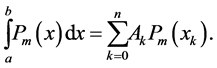
Usually, the approximate value of the integral is calculated using the so-called formulas for numerical integration or quadrature formulas. The general idea is to approximate the integral as a sum
 (5)
(5)
of the values of the function , calculated at some nodes
 , multiplied by some coefficient
 , called weights or weight coefficients. The nodes and the weight coefficients do not depend on the function
 .
.
Usually the nodes and the weight coefficients are calculated so that the formula is exact for the polynomials of highest possible degree. We say that the quadrature formula is exact for all polynomials of degree  if for any polynomial
  of degree
 (6)
(6)
In this work we consider so called Newton-Cotes formulas defined on a fixed set of nodes ,
,  (see [3] for details). In this case, in order to obtain the coefficients
 , one has to solve the system of linear equations
 (7)
(7)
The Error Term
The error term,  , is defined as
 (8)
(8)
If the function  has a continuous
  derivative, the error term can be represented in the form (see for details [3] [4] )
 (9)
(9)
where  is a constant and
 .
.
The degree of precision of a quadrature formula is defined as the positive integer  satisfying
  for
for , where
  is a polynomial of degree
 , but
, but  for some polynomial of degree
 .
.
2. Midpoint Rule
The simplest formula, using only one node, is the Midpoint Rule. Suppose the node is the midpoint
 of the interval
 . By solving the Equation (7), we obtain the formula
 (10)
(10)
If the function  has a continuous second derivative, the error term of the Midpoint Rule can be represented in the form
 (11)
(11)
where .
.
2.1. Composite Midpoint Rule
In order to reduce the error term we partition the interval  into
into  subintervals
 ,
,
 . Assume
 ,
,  , and
, and  (see Figure 1). Suppose the length of each subinterval is the same,
 . So,
. So,  and
and . Then,
 (12)
(12)
If the function  has a continuous second derivative in
 , the approximation error
 (13)
(13)
is given as
 (14)
(14)
where .
.
Suppose we have performed two calculations with different numbers of subintervals,  and
and . Then
 (15)
(15)
and
 (16)
(16)
If , we obtain
 (17)
(17)
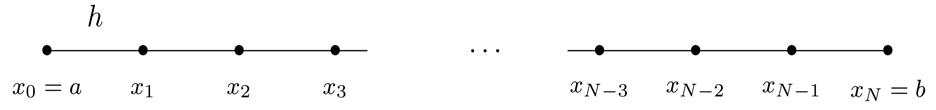
Figure 1. The mesh.
Therefore, if we double the number of subintervals, the error term is decreased four times. This is a practical way of confirming the power of  in the error term. In practice [5] , the ratio is not exactly four, because
  is usually not constant.
2.2. Numerical Experiments
We prepared a SAGE function MPloop for our numerical experiments with the Midpoint Rule. The code is given here:
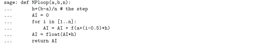
The variables a and b are the lower and upper limits of the integral, and the variable n is the number of subintervals.
The results obtained with the function MPloop for the integral
 (18)
(18)
are shown in Table 1. The last column shows the ratio of the errors . Our numerical calculations confirm that if we double the number of subintervals, the error term is decreased four times. The error distribution for the same calculation is given in Figure 2. The red dots are the numerical error and the blue line is the graph of the function
 . Again, the numerical experiments confirm that the error is going to zero when
  is going to infinity the same way as the function
  is going to zero. One application of the Midpoint Rule can be found in [6] .
3. Trapezoidal Rule
The formula based on two nodes,  and
and , and exact for all second order polynomials, can be calculated via the system of two Equations (7). The resulting formula
 (19)
(19)
is called Trapezoidal Rule, because it produces exactly the area of the trapezoid with vertexes ,
,  ,
,  , and
, and .
.
If the function  has a continuous second derivative, the error term of the Trapezoidal Rule can be represented in the form (see [3] )
 (20)
(20)
where .
.
3.1. Composite Trapezoidal Rule
The composite formula for the Trapezoidal Rule is
 (21)
(21)
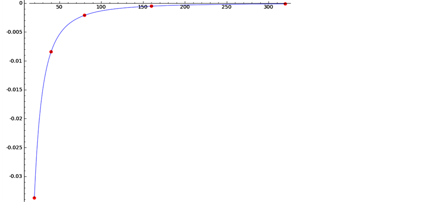
Figure 2. The error distribution for 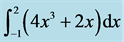 calculated with Midpoint Rule. The red dots are the errors and the blue curve is
 .
.

Table 1. Numerical results for  calculated with the Midpoint Rule.
The nodes  are defined in subsection 2.1 as given in Figure 1.
The error term is (see [5] for details)
 (22)
(22)
where .
.
As with the Midpoint Rule, we obtain
 (23)
(23)
3.2. Numerical Experiments
We construct a SAGE function TPloop(a,b,n) for the composite Trapezoidal Rule:
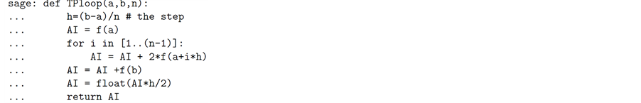
The variables a and b are the lower and upper limits of the integral, and the variable n is the number of subintervals.
The results obtained with function TRloop for the integral (18) are shown in Table 2. The last column shows the ratio of the errors . Our numerical calculations confirm that if we double the number of subintervals, the error term is decreased four times. The error distribution for the same calculation is shown graphically in Figure 3. The graph of the function
  is given in the same figure. The error points and the graph of the quadratic function are undistinguishable. This experiment confirms the second order of approximation of the numerical realization of the Trapezoidal Rule.
4. Simpson’s Rule
Suppose we want to use three nodes ,
,  , and
, and . For this case the quadrature Formula (5)
has three free (unknown) coefficients

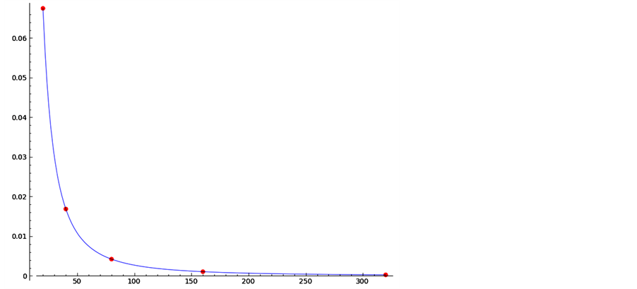
Figure 3. The error distribution for  calculated with the Trapezoidal Rule. The red dots are the errors and the blue curve is
  .
.
Table 2. Numerical results for  calculated with the Trapezoidal Rule.
and we can make the formula exact for second order polynomials. In other words, the formula must be exact for all polynomials of zero degree and particularly for . So,
. So,

The formula must be exact for all first order polynomials and particularly for . Therefore,

The formula must be exact for all second order polynomials and particularly for . Therefore,

The last three equations form the system (7) for this case. The solution to the system is ,
,  , and the Simpson’s Rule is given by
 (24)
(24)
The error term, under the condition that the fourth derivative  of the function
  exists and is continuous in the interval
 , is given by (see [5] )
 (25)
(25)
4.1. Composite Simpson’s Formula
One way to construct the composite Simpson’s formula is to divide the interval  into an even number of subintervals, say
 . Then the composite formula is
 (26)
(26)
where . The error term in this case is
 (27)
(27)
where .
.
As with the two previous rules, we obtain
 (28)
(28)
So, if the number of subintervals is multiplied by 2, the numerical error decreases by a factor of .
.
4.2. Numerical Experiments
We prepared a SAGE function Simpsons for our numerical experiments with Simpson’s Rule. The code is given here:
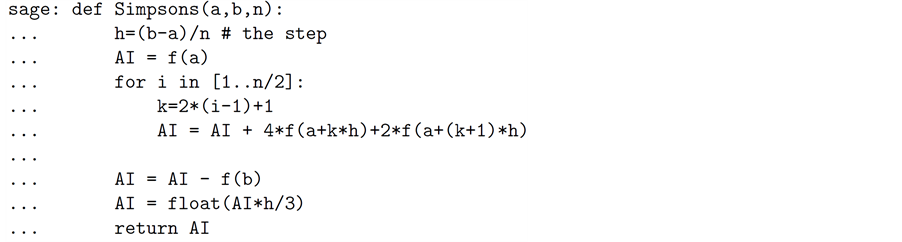
The variables a and b are the lower and upper limits of the integral, and the variable n is the number of subintervals.
The results obtained with function Simpsons for the integral
 (29)
(29)
are shown in Table 3. The last column shows the ratio of the errors . Our numerical calculations confirm that if we double the number of subintervals, the error term decreases sixteen times. The error distribution for the same calculation is given in Figure 4. The red dots are the numerical error and the blue line is the graph of the function
 . Because the error approaches zero very rapidly, we use a logarithmic scale on the
  -axis. The numerical experiments confirm that the numerical error’s rate of approach to zero as
 approaches infinity is the same as the rate of approach to zero of the function
 .
.
5. Error Estimation from Numerical Results
How do we determine the number of subintervals such that the computed result meets some prescribed accuracy?
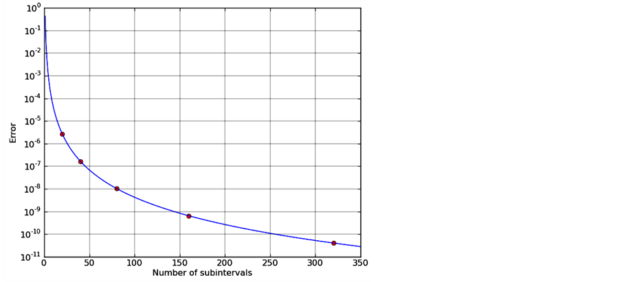
Figure 4. The error distribution for  calculated with composite Simpson’s Rule. The red dots are the errors and the blue curve is
 .
.
Table 3. Numerical results for  calculated with Simpson’s Rule.
According to the formulas for the error (14), (22), and (27), the error depends on a derivative of the integrand. If we know the corresponding derivative of the integrand, we can calculate the upper bound of the error. Usually, in practice we do not know the relevant derivative of the integrand and we cannot bound the error this way.
In practice, we frequently use the rule known as Runge’s principle. The formulas for numerical integration (12), (21), and (26) are of the form
 (30)
(30)
where  is the approximated value of the integral calculated when the interval
  is divided into
  subintervals, and
 (31)
(31)
is the error term for the corresponding formula,  is a constant,
  are integers, and
 .
.
Suppose we perform two calculations with different numbers of subintervals,  and
and :
:
 (32)
(32)
Under the assumption  (see [5] for details), we can eliminate
  from the above two equations, to obtain
 (33)
(33)
This approximation of the error term is known as Runge’s principle. In addition, instead of , we can use
 (34)
(34)
as a better approximation of the integral. This technique is known as Richardson’s extrapolation; it is used in many types of numerical calculations, especially when we are solving differential equations numerically.
In practice, usually the exact value of the integral  is unknown. So, we cannot use the Formulas (17), (23), and (28) to confirm the power of
  in the error term. Substituting
  with
with  from the Runge principle, we obtain
 (35)
(35)
Next we will consider the Runge principle, Richardson’s extrapolation, and the power of  estimation in the error term to the Midpoint, Trapezoidal, and Simpson’s rules.
5.1. Midpoint Rule
A simple SAGE implementation of the Runge principle for estimating the error during the numerical calculations is given here:
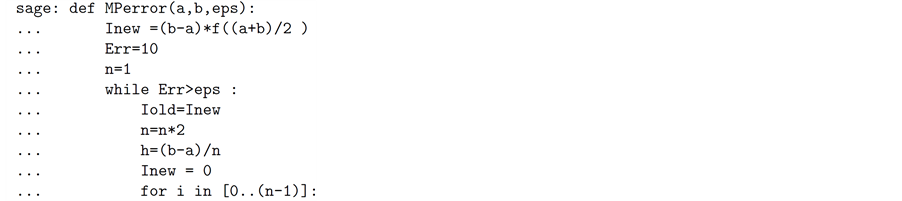

The variables a and b in the definition of the function MPerror contain the lower and upper limits of the integral. The variable eps is the satisfactory error. The function returns: the first variable, Inew, is the approximation of the integral with the Midpoint Rule; the second variable, Iextr, is the value of Richardson’s extrapolation for the integral using Iold and Inew; the third variable n gives the number of subintervals for the final approximation.
To verify the theoretical results for the Midpoint method, we calculate the integral
 (36)
(36)
with a different number of subintervals, and approximate the value of the integral with Richardson’s extrapolation. The results are given in Table 4. Our numerical experiments confirm the second order of approximation  of the Midpoint Rule, and show that Richardson’s approximation has a fourth order of approximation
  of the integral.
5.2. Trapezoidal Rule
When the number of subintervals  increases, the error in the composite Trapezoidal Rule reduces. On the other hand, when
  increases, the number of the function values to be calculated also increases. We need to find a balance between the accuracy requirements and the cost (in operations or computing time) of the algorithm. This balance can be reached with the following algorithm:
We calculate the approximation of the integral  by applying the Trapezoidal Rule over the whole interval
 . Then we calculate the approximation
  by dividing the interval
  into two subintervals, and in each we apply the Trapezoidal Rule. In this partition the new node is only one in the middle of this interval. The other two nodes are involved in the calculation of
  and we do not need to calculate the value of the function on those nodes again. We calculate
  by introducing four subintervals. The new nodes are only two. So, we find
 , such that the number of subintervals needed to calculate
  is
is , but the number of new nodes of the mesh on which we calculate
  is
is . The remaining
  nodes are involved in the calculation of
 , and the values of the integrand are already calculated. The process continues until the following condition holds:
Table 4. Numerical error for the Midpoint Rule, Richardson’s extrapolation, and the rates of convergence.

This algorithm is an example of the so-called adaptive algorithms the number of required subintervals depends on the integrand, but the step is uniform throughout the interval . Sometimes we need to use a mesh with different steps depending on the behavior of the function under the integral.
A simple SAGE implementation of the Runge principle for estimating the error during the numerical calculations with Trapezoidal Rule is given here:
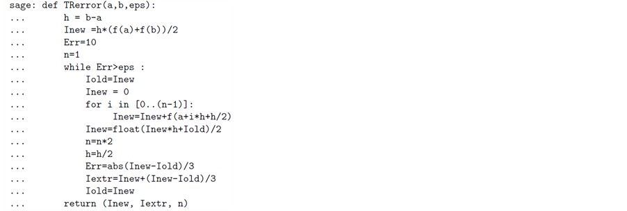
The variables a and b in the definition of the function TRerror contain the lower and upper limits of the integral. The variable eps is the satisfactory error. The function returns: the first variable, Inew, is the approximation of the integral with Trapezoidal Rule; the second variable, Iextr, is the value of Richardson’s extrapolation for the integral using Iold and Inew; the third variable n gives the number of subintervals for the final approximation.
To verify the theoretical results for the Trapezoidal method, we calculate the integral (36) with a different number of subintervals and approximate the value of the integral with Richardson’s extrapolation. The results are given in Table 5. Our numerical experiments confirm the second order of approximation  of the Trapezoidal Rule and show that Richardson’s approximation has forth order of approximation
  of the integral.
The fact that Richardson’s extrapolation applied to the Trapezoidal Rule gives fourth order of approximation has a simple explanation. Since,
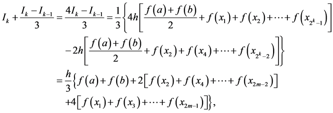 (37)
(37)
Table 5. Numerical error for the Trapezoidal Rule, Richardson’s extrapolation, and the rates of convergence.
Richardson’s extrapolation for the Trapezoidal Rule is nothing else but Simpson’s formula. Our numerical experiments show that the error term for Richardson’s extrapolation is the same  as the error term for Simpson’s formula.
5.3. Simpson’s Rule
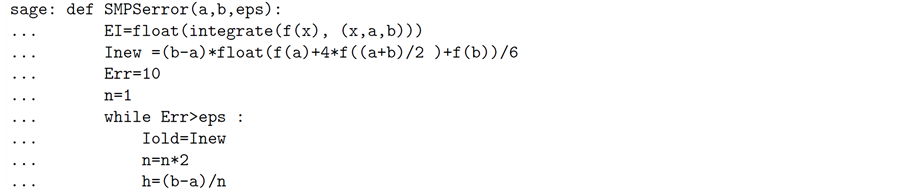
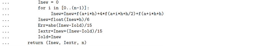
To verify the theoretical results for Simpson’s method, we calculate the integral (36) with a different number of subintervals, and approximate the value of the integral with Richardson’s extrapolation. The results are given in Table 6. Our numerical experiments confirm the fourth order of approximation  of Simpson’s rule, and show that Richardson’s approximation has a sixth order of approximation
  of the integral. The SAGE code is given here:
6. Adaptive Procedures
According to [5] : “An adaptive quadrature routine is a numerical quadrature algorithm which uses one or two basic quadrature rules and which automatically determines the subinterval size so that the computed result meets some prescribed accuracy requirement.’’ For our adaptive function we chose the Midpoint Rule, because it involves just one node to approximate the integral in the given subinterval. The SAGE function needs to be changed slightly if one wishes to use a different quadrature formula. The SAGE code for the function MPrecursion(a,b,eps) is given here:
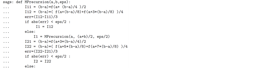

The parameters of the function MPrecursion are a and b-the lower and upper limits of the integral, and eps the accuracy. The function divides the interval into two subintervals, and, in each subinterval, approximates the integral twice using the Midpoint Rule for the full half interval and using the composite Midpoint Rule, which divides the half interval into two subintervals. If the error, according to Runge’s principle, is less than eps, the value calculated with the composite rule is accepted as an approximation of the integral for this subinterval. If
Table 6. Numerical error for Simpson’s rule, the Richardson’s extrapolation, and the rates of convergence.
the error is greater than the prescribed accuracy, the function calls itself with a half-length interval and halved accuracy requirements. Therefore, we have one recursive algorithm which uses different mesh sizes for different parts of the interval. If the integrand is smooth and slowly varying, a relatively small number of subintervals is used. In the parts of the interval where the integrand is changing rapidly, the mesh is relatively fine.
An example of the behavior of the function MPrecursion is given in Figure 5. The red dots on the  -axis are the nodes used for calculation of
 (38)
(38)
and the blue line is the graph of the integrand.
7. Can We Always Trust the Runge Principle?
As we have shown in the previous section, the Runge principle for estimating the error during the numerical calculations works well under the condition that the respective derivative of the integrand exists and this derivative is a continuous function. If the derivative in the error term does not exist, the Runge principle fails, and Richardson’s extrapolation cannot be applied. Consider the following examples.
7.1. Improper Integrals
The formal definition of improper integral is:
If  when
when  (or
(or  when
when ), then
 (39)
(39)
Examples:
 (40)
(40)
Calculating improper integrals numerically is challenging. Usually, we need some a priori information about the integrand, because the techniques we apply depend on the properties of this function. Two main problems arise:
1) the integrand is not defined at one (or both) limits of the integral;
2) the integrand goes to infinity at one (or both) limits of the integral;
Because of 1) Trapezoidal and Simpson’s rules cannot be used. The Midpoint Rule can be used, since we do not need the value of the function at the endpoints  and
and .
.
The results from calculations of the first improper integral from (40) with the Midpoint Rule are given in Table 7. The ratio of the errors in this case is about 1.414. Compared to the ratio of 4 for the “good’’ functions, we see that the convergence is very slow. We will have a similar convergence for a “good’’ integrand when we approximate the integral with a formula with error term .
.
7.2. Singularity in the Derivative
The slow convergence of the improper integral is not a surprise, since the integrand goes to infinity at one of the endpoints of the interval. Consider the integral
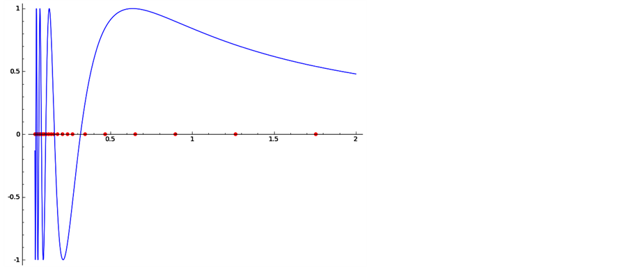
Figure 5. The mesh used from the adaptive algorithm to approximate.
Table 7. Numerical results for  calculated with the Midpoint Rule.
 (41)
(41)
The function  is a continuous and bounded function, but the second derivative of this function goes to infinity when
 . So, we can expect problems with practical convergence of the numerical calculation of the integral. The results from the numerical calculations of (41) with the Midpoint Rule are given in Table 8. The ratio of the errors in this case is about 2.8. Comparing this ratio to 4, for the “good’’ functions, we see that the convergence is slow. We will have a similar convergence for a “good’’ integrand when we approximate the integral with the formula with error term
 .
.
8. Behavior of the Error in Practice
We have to emphasize that in practical calculations the error in the final result depends on the accumulation of rounding errors. With the increasing number of subintervals the theoretical error decreases, but the number of arithmetic operations, each of which contains an error in the order of machine epsilon, increases. Therefore it is reasonable to use as many subintervals as we need to get the theoretical error term to exceed the machine epsilon. The total error starts to increase when the number of subintervals increases beyond a certain unknown number dependent on the integrand, the programming language, and the computer.
To illustrate this effect with our SAGE codes we use the class RealField with 32 bits. The effect when the Sage 64-bit floating-point system is used is similar but the computing time increases. The numerical results for three integrals,
 (42)
(42)
are shown in Figure 6. When the number of subintervals is relatively small, the error decreases as the number of subintervals increases. When the number of subintervals becomes greater than a certain number, the error start to increase. The number after which the error start to increase depends on the integrand.
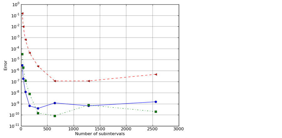
Figure 6. The error behavior for  the blue solid line,
 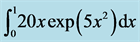 the red dashed line, and
  the green dashdot line.
Table 8. Numerical results for  calculated with Midpoint Rule.
Acknowledgements
This work was supported by NSF grant HRD-0928797.
References
- Marinov, T.T. and Marinova, R.S. (2010) Coefficient Identification in Euler-Bernoulli Equation from Over-Posed Data. Journal of Computational and Applied Mathematics, 235, 450-459. http://dx.doi.org/10.4153/CJM-1969-153-1
- Marinov, T.T. and Vatsala, A. (2008) Inverse Problem for Coefficient Identification in Euler-Bernoulli Equation. Computers and Mathematics with Applications, 56, 400-410. http://dx.doi.org/10.1112/blms/25.6.527
- Ackleh, A.S., Kearfott, R.B. and Allen, E.J. (2009) Classical and Modern Numerical Analysis: Theory, Methods and Practice, Chapman & Hall/CRC Numerical Analysis and Scientific Computing. CRC Press, Boca Raton. http://dx.doi.org/10.1142/S0218196791000146
- Press, W.H. and Teukolsky, S.A. and Vetterling, W.T. and Flannery, B.P. (2007) Numerical Recipes: The Art of Scientific Computing. Cambridge University Press, New York. http://dx.doi.org/10.1142/S0218196799000199
- Forsythe, G.E. and Malcolm, M.A. and Moler, C.B. (1977) Computer Methods for Mathematical Computations. Prentice Hall Professional Technical Reference, Upper Saddle River. http://dx.doi.org/10.1051/ita/2012010
NOTES

*Corresponding author.