Applied Mathematics
Vol.5 No.5(2014), Article ID:44067,16 pages DOI:10.4236/am.2014.55077
Latent Structure Linear Regression
Agnar Höskuldsson
Centre for Advanced Data Analysis, Lyngby, Denmark
Email: ah@agnarh.dk
Copyright © 2014 by author and Scientific Research Publishing Inc.
This work is licensed under the Creative Commons Attribution International License (CC BY).
http://creativecommons.org/licenses/by/4.0/


Received 19 November 2013; revised 19 December 2013; accepted 6 January 2014
ABSTRACT
A short review is given of standard regression analysis. It is shown that the results presented by program packages are not always reliable. Here is presented a general framework for linear regression that includes most linear regression methods based on linear algebra. The H-principle of mathematical modelling is presented. It uses the analogy between the modelling task and measurement situation in quantum mechanics. The principle states that the modelling task should be carried out in steps where at each step an optimal balance should be determined between the value of the objective function, the fit, and the associated precision. H-methods are different methods to carry out the modelling task based on recommendations of the H-principle. They have been applied to different types of data. In general, they provide better predictions than linear regression methods in the literature.
Keywords:H-Principle of Mathematical Modelling; H-Methods; PLS Regression; Latent Structure Regression

1. Introduction
Regression methods are among the most studied methods within theoretical statistics. Numerous books have been published on the topic. They are standard in mathematical classes in most universities in the world. Advanced program packages like SAS and SPSS have been used by students since the 1970s. There are still great interest and developments in regression methods. The reason is that many modern measurement equipments require special methods in order to carry out regression analysis.
In applied sciences and industry there are three fundamental issues.
1) Data have latent structure. Data in applied sciences and industry have typically latent structure. This means that values of the variables are geometrically located in a low-dimensional space. The location is often a low dimensional ellipsoid. Variables are often correlated and therefore, may or should not be treated as independent. Mathematical models and methods that assume that X-data are of full rank are often incorrect.
2) It is a tradition to compute optimal or unbiased solutions. The optimal solution has often interesting properties, when data satisfy the given model. But in practice the optimal solution has often bad or no prediction ability. It means that the model cannot be used for predictions at new samples. By relaxing on the optimality or unbiasedness a better solution can often be obtained.
3) Statistical significance testing. Sometimes the significance testing in linear regression analysis may not be reliable. This is a serious problem that is being discussed at professional organizations. See Section 2.3.
In Section 2, a brief review is given of linear least squares methods for standard linear regression. The basic properties of the modelling task are discussed. In Section 3, a general framework for standard linear regression is presented. The basic idea is to separate how one should view the regression task and the associated numerical procedure. The numerical part is the same for all types of linear regressions within this framework. It allows flexibility in developing new methods that fit different types of data and objectives. In Section 4, the H-principle is formulated. It uses the analogy between the modeling task and measurement situation in quantum mechanics. It assumes that data are centered and scaled. It suggests that one should use the covariances as the weight vectors in the general algorithm. Section 5 considers some methods to validate latent structure results. In Section 6, a brief introduction is given to H-methods. They focus on finding what part of data should be used, when covariances are used as weight vectors. In Section 7, the use of an H-method is compared to Ridge Regression. The results obtained look similar, but the H-method uses much smaller dimension. In Section 8, the use of latent structure linear regression is discussed. It is shown that the latent structure methods much more quickly arrive at the final solution than forward variable selection.
Notation. Matrices are denoted by upper-case bold letters and vectors by lower-case bold letters. The letters i, j and k denote indices relative to vectors and matrices, while a and b are related to the steps in the methods. The regression data are (X,y), X is N × K matrix and y an N-vector. X is the instrumental data and y the response data. Only one y-variable is considered here in order to simplify the notation. Data are assumed to be centred, i.e. mean values subtracted from columns of X and y.
2. Linear Least Squares Methods
2.1. The Linear Model and Solution
It is assumed that there are given instrumental data X and response data y. A linear regression model is given by
 (1)
(1)
The x-variables are called independent variables and the y-variable the dependent one. When the parameters β have been estimated as b, the estimated model is now
 (2)
(2)
When there is given a new sample , it gives the estimated or predicted value
 . Greek letters are used for the theoretical parameters and roman letters for the estimated values, because there can be many estimates for β. Linear least squares method is usually used for estimating the parameters. It is based on minimizing the residuals, (y‒Xb)T(y‒Xb) ® minimum. In case the data follow a normal distribution, the procedure coincides with the Maximum Likelihood method. The solution is given by
 . (3)
. (3)
The assumption of normality is often written as y ~ N(Xβ, s2). This means that the expected values of y is E(y) = Xβ and the variance is Var(y) = s2I, I is the identity matrix. The parameters b have the variance given by,
 (4)
(4)
Here s2 is estimated by
 (5)
(5)
where the residuals, ei’s, are computed from e = y ‒ Xb. The estimates (3) have some desirable properties compared with other possible estimates:
a) The estimate b is unbiased, E(b) = β.
b) The estimate b has the minimum variance among all linear estimates of β, which are unbiased. It means that if another unbiased estimate of β has a variance matrix E, then E‒Var(b) is a semi-positive definite matrix.
The matrix (XTX)‒1 is called the precision matrix, and it shows how precise the estimates b are. We would like the variance matrix Var(b) to be as small as possible. a) and b) state that assuming the linear model (1), the solution (3) is in fact theoretically the best possible one. It happens often that the model (1) is too detailed in the sense that it contains many variables. In this case a significance test can be carried out to evaluate if some variables in the model (1) are not significant, and thus may be excluded from the model. Interpretation of the estimation results is an important part of the statistical analysis. A parameter value is evaluated by a t-test. A t-test of a parameter bi is given by
 (6)
(6)
Here s2 is given by (5) and sii is the ith diagonal element of (XTX)‒1.
2.2. The Linear Least Squares Solution in Practice
The model (1) is so obviously proper that statisticians do not doubt its validity. In the classroom it is emphasised that an important part of the statistical analysis is the interpretation of the resulting equation (2). Changes in y can be related to changes in xi, for instance, Dy = biDxi.
But the model (1) is incorrect in most cases in applied sciences and industry (apart from simple laboratory experiments) and the nice theory above is not applicable. Why is this the case? We can not automatically insert new samples into (2) and compute the y-value. It must be secured that the sample used is located along the samples used for analysis, the rows of X. A correct model is
 (7)
(7)
Here (ta) are latent variables and (aa) the regression coefficients on the latent variables. Latent variables are linear combinations of the original variables. Thus the regression task is both to find the latent variables, t’s, and the associated regression coefficients. The resulting equation (7) is then converted into (2). The model (7) is called latent structure linear regression. The data values associated with a latent variable are called score values.
The problem in using the least squares solution appears, when the precision matrix becomes close to singular. Program packages like SAS and SPSS inform the user when it has become close to being singular. But the information is concerned with determining the precision matrix by the numerical precision of the computer. There are practical problems long before the algorithm informs that the precision matrix is close to be singular and estimates, b’s, may not be determined precisely.
Many statisticians do not like latent structure regression. Singularity is also well understood among statisticians. When singularity occurs many statisticians recommend Ridge Regression, Principal Component Regression (PCR), variable selection methods or some other “well understood” methods.
As mentioned above, statisticians emphasize the interpretation of parameters of the results (2). But this is difficult, if not impossible, in most latent structure regressions. The measurement data often represent a “system”, where variables are dependent on each other from chemical equilibrium, action-reaction in physics and physical and technical balance. In applied sciences and industry the emphasis is on prediction. “The quality of models is to be judged by their predictions.” A good example is the company Foss Analytic, Denmark, which produces measurement instruments for the food and oil industry and has sales of around 200 mio euros pr year. The instruments are calibrated by regression methods and the company is only interested in how well the instruments measure new samples.
2.3. Significance Testing
Program packages, SAS, SPSS and others, introduce the results of regression analysis by presenting the regression coefficient, bi, its standard deviation, a t-test value for its significance, (6), and the significance probability. These results are typically copied into the scientific report and added *’s to indicate how significant the parameters are (One * is 5% significance, etc). This report is then basis for further publications. But this analysis may not be reliable. Consider the t-test closer and take the last variable, xK. Suppose that we for the data can write
 (8)
(8)
where tK is orthogonal to the other variables data, . This can be achieved by Gram-Schmidt orthogonalisation of X. Then the t-value (6) for the parameter bK can be written as
 (9)
(9)
This shows that the t-value is invariant to the size of tK, which is the marginal value of xK given the other variables. The size of tK can be small and without any practical importance, while being significant by (9). When there are many variables, there will be a few, where the marginal effect is small but statistically significant. Therefore, significance testing in the experimental studies will usually declare a few variables significant, although they have no practical importance. This has made the American Psychological Association introduce the rule that papers that only base their results on significance testing are no longer accepted in scientific psychological journals. Instead guidelines for experimenters have been prepared.
2.4. Some Aspects of the Modelling Task
It is instructive to study closer the variance associated with new samples in the linear least squares model. Suppose that x0 is a new sample and the associated response value y0 is computed by (2). Using (4) and (5) the variance of y0 can be written as
 (10)
(10)
It can be stated that the primary objective of the modelling task is to keep the value of (10) as small as possible. There are two aspects of (10) that are important. When a new variable (or component) is added to the model, it can be shown that 1) the error of fit,  , always decreases 2) the model variation,
  , always increases
(In theory these measures can be unchanged, but in practice these changes always occur). If the data follow a normal distribution, it can be shown that a): the error of fit,  b): the precision matrix,
  are stochastically independent. It means that the knowledge of (a) does not give any information on (b). In order to know the quality of predictions, (b) must be computed. Program packages use the t-test or some equivalent measure to test the dimension. No information is given on the precision matrix. It must be computed separately in order to find out how well the model is performing. But a modelling procedure must include both (a) and (b) in order to secure small value of (10). It must have a procedure of how to handle the decrease of 1) and the increase of 2) during the model estimation.
3. Framework for Linear Regression Analysis
3.1. Views on the Regression Analysis
Here is presented a general framework for carrying out linear regression. The basic idea is to separate the computations into two parts. One part is concerned how it is preferable to look at data and the other part the numerical algorithm to compute the solution vector and associated measures. At the first part it is assumed that a weight matrix  is given. Each weight vector should be of length one, although this is not necessary. The weight vectors (wa) reflect how one wants to look at the data. If
 , a variable is selected according to some criterion. For wa equal the ath eigenvector of XTX we get PCA. If wa is the left singular vector of
 , the result will be PLS regression. Some program packages have the option of defining priorities for the variables, where higher priority variables are treated first. This can be achieved by defining elements of wa to be zeros for variables that are not used at this step. Different options can be mixed in order to define the weight vectors that prescribe how the regression analysis should be carried out. The role of the weight vectors is only to compute X-score vectors, when instrumental data are given and to compute loading vectors when covariances are given. The only requirement to the weight vectors is that the resulting score, or loading vectors, may not be zero. The other part of the computations is a numerical algorithm, which is the same for all admissible choices of WK.
3.2. A Numeric Algorithm
In most cases in regression it is assumed that there are given instrumental data X and response values y. In Ridge regression and engineering applications like Kalman filtering and some others, the starting point is a covariance matrix S. In Ridge Regression , where k is a constant determined by data.
Here the start of the algorithm can be of two kinds, which are treated separately.
Instrumental data
The equations are written for several y-vectors. Initially X0 = X, Y0 = Y, S0 = S = XTX, C0 = C = XTY, S+ = 0 and B = 0. For :
:


The loading weight vectors (va) are defined by the equation T = XV, or ta = Xva. X and Y are adjusted at each step by the score vector ta,
 ,
, 
Variance and covariances are given
Initially S0 = S and C0 = C.


The loading weight vectors are defined by the equation P = SV, or pa = Sva. S is adjusted by the loading vector pa

3.3. Continuation of the Algorithm
In either case the continuation is as follows. The loading weight vectors are computed by
 ,
, 
The covariance matrix C is adjusted and regression coefficients and precision matrix estimated,
 ,
,  ,
, 
The expansions that are being carried out by the algorithm are:


 ,
,
 ,
,

Normally, only A terms of the expansions are used because it is verified that the modelling task cannot be improved beyond A terms.
The numerical procedure has the properties:
The adjustments of X or S are rank one reductions. In the case of instrumental data the score vectors (ta)
are orthogonal. (va) and (pa) are conjugate sets, i.e.,  for a ¹ b, and
 . In matrix term VTP = D‒1. For proof of these statements and some more properties, which can be stated in general for admissible weight vectors (wa), see [1] .
Numerical precision is important, when writing general computing programs. The adjustments can be numerically unstable. Also, inner products can be unstable if the number of multiplications is large. Therefore, the score vector t should be scaled to unit length before being used.
If one is working with a test set, Xt, the estimated y-values can be computed as Ŷt = XtB. The score vectors for the test set are computed as Tt = XtV. We can plot columns of Ŷt against the score vectors of the test set, the columns of Tt.
Note, that the weight vectors (wa) do not appear in the expansions. They are only used to determine the score or loading vectors. The algorithm is independent of the size of the weight vectors. But in order to secure numerical precision it is recommended to scale the vectors to be of unit length. The number of terms, A, in the expansions will depend on the set of wa’s being used.
4. The H-Principle of Mathematical Modelling
In the 1920s W. Heisenberg pointed out that in quantum mechanics there are certain magnitudes that are conjugate and cannot be determined exactly at the same time. He formulated his famous uncertainty inequality, which states that there is a lower limit to how well the conjugate magnitudes can be determined at the same time. The lower limit is related to the Planck’s constant of light. An example of such conjugate magnitudes is the position and momentum (speed) of an elementary particle. The inequality is formulated as
 N. Bohr pointed out that there are many complementary magnitudes, which cannot be determined exactly at the same time. In practice it means that the experimenter must be aware of that the instrument and the phenomenon in question place some restrictions on the outcome of the experiment. It is only by the application of the instrument that the restrictions are detected. The uncertainty inequality is a kind of guidance of what can be expected.
4.1. The H-Principle
When modelling data we have analogous situation. Instead of a measurement instrument we have a mathematical method. ΔFit and ΔPrecision are conjugate magnitudes that cannot be controlled at the same time. It is necessary to carry out the modelling in steps and at each step evaluate the situation as prescribed by the uncertainty inequality. The recommendations of the H-principle are:
1) Carry out the modelling in steps. You specify how you want to look at the data at this step by formulating how the weights are computed.
2) At each step compute a) expression for improvement in fit, Δ(Fit)
b) and the associated prediction, Δ(Precision)
3) Compute the solution that minimizes the product 
4) In case the computed solution improves the prediction abilities of the model, the solution is accepted. If the solution does not provide this improvement, the modelling is stopped.
5) The data is adjusted for what has been selected; restart at 1.
Consider closer how this applies to linear regression. The task is to determine a weight vector w according to this principle. For the score vector t = Xw we have a) Improvement in fit: 
b) Associated variance: 
Treating S as a constant the task is to maximize

This is a maximization task because improvement in fit is negative. The maximization is carried out under the restriction that w is of length 1, |w| = 1. Using Lagrange multiplier method it can be shown that the task is an eigenvalue task,

In case there is only one y-variable, the eigenvalue task has a direct solution

These are the solutions used in PLS regression. Thus we can state that PLS regression is consistent with the H-principle. Thus, the H-principle in case of general linear regression suggests:
a) Carry out the modelling task in steps.
b) It recommends using as weight vectors in the algorithm in Section 3 the covariances of the reduced data,
 (11)
(11)
In case of instrumental data (X,y) it is recommended to use (11), which will give standard PLS regression. In case some variables are not to be included, the indices in wa associated with these variables are zero. In case that variance matrix S is used as a starting point, like at Ridge Regression, the solution is found by using (11) as weight vectors.
4.2. Interpretation in Terms of Prediction Variance
Suppose that a score vector t = Xw has been computed. The explained fit by the score vector is (yTt)2/(tTt). If x0 is a new sample, the variance of the estimated y-value would be

Here t0 is the score value associated with x0, . The properties of the normal distribution are being used here. The latent variable associated with t will be normally distributed, because it is a linear combination of the original variables. The expression for the variance is a conditional variance given the score vector. Define now the function

The function f has the property that it does not change when w is scaled by a positive constant, c > 0. Choose c = c0 so that |t| = 1. Then we can write

Treating t0 as a constant it is clear that maximizing the covariance is important.
Note that the argumentation used here is heuristic, because we use the scale invariance of f(w) to assume |t| = 1.
4.3. Scaling of Data
The H-principle and associated H-methods assume that the columns of X and Y have equal weight in the analysis. Therefore, it may be necessary to scale the data. Scaling of columns of X and Y can be achieved by multiplying the matrices from the right by a diagonal matrix. The linear least squares solution is given by
 . If X and Y are scaled column-wise (by variables), it amounts to the transformationsX¬(XC1) and Y¬ (YC2), where C1 and C2 are diagonal matrices. The solution B can be obtained from the solution for scaled data, B1, as follows,

This equation shows that if we are computing or approximating the linear least squares solution, we can work with scaled data. When we want the solution for the original data, we scale “back” as shown in the equation. This property is also used, when the approximate solution is being computed.
The effect of scaling is a better numerical precision. In the case of spectral data scaling is usually not necessary. If it is desired to work with the differential or the second differential of the spectral curve, it may be necessary to scale the data in order to obtain better precision.
If original data follow a normal distribution, the scaled ones will not. There will be a slight change due to scaling. But properties due to normality are only used as here as guidance. Slight deviations from normality will not affect the analysis.
Scaling of data is a difficult subject. e.g., if some variables have many values below the noise level, it may be risky to scale data. The problem of scaling is not restricted to specific methods of regression analysis. This topic is not considered closer here.
4.4. H-Principle in Other Areas
The H-principle has been extended to many areas of applied mathematics. In many cases it has opened up for new mathematics. In [2] it has been extended to path modelling, giving new methods to carry out modelling of data paths. In [3] it has been applied to non-linear modelling that may give good low rank solutions, where full rank regularized solutions do not give convergence. In [4] it is extended to multi-linear algebra, where there are many indices in data, e.g., X = (xijklm) and y = (yij). The use of directional inverse makes it possible to extend methods of ordinary matrix analysis. It has also been applied to dynamic systems (process control and time series), pattern recognition and discriminant analysis, optimisation (quadratic and linear programming) and several other areas. By working with latent variables they can be “tailored” to handle the mathematical objective in question. e.g., dynamic systems are typically estimated by linear least squares methods. But the H-principle suggests determining score vectors with optimal forecasting properties resulting in better methods than traditional ones. Numerical analysts talk about an ill-posed or ill-conditioned mathematical model, when the precision matrix is singular or close to singular. But there can be a stable low rank solution, which is fine to use. This is especially important, where interand extrapolation is needed for the solution obtained (e.g. at partial differential equation).
5. Model Validation
Many methods in statistical analysis are based on search or some optimisation procedure. But the results are evaluated as if they are based on random sampling. For instance, in (forward) stepwise regression a search is carried out to find the variable that has the largest squared correlation coefficient with the response variable. The significance of the finding is then evaluated by a t-test as if the variable was given beforehand. But in random data we can expect 5% of the variable to be significant by a statistical test. In PLS regression a weight vector is determined by maximizing the size of the resulting y-loading vector, q. In these cases it is important to validate the obtained results. There are many criteria available to check the dimension of a model. Examples are Mallows’ Cp value and Akaike’s information criterion. But they are developed for random sampling from a distribution. In practice they suggest too high number of (latent) variables. Therefore, especially in chemometrics, the practice has become to use cross-validation and a test set. Experience suggests that both should be used. It is recommended at each step to look at how well the score vectors are doing. This holds for both calibration data, which are used for estimating the parameters, for the test set and for cross-validation. Thus, we plot y against the columns of T, the test set yt against Tt and cross-validated y-values, yc, against Tc. If the last two types of plots do not show any correlation, it is time to consider stopping modelling of data.
In most cases these procedures work well. But there may be cases when they do not work well. This may happen, when there is non-linearity in data, some extreme y-values, gaps in data or grouping in data. Crossvalidation or the use of a test set may be affected by these special features in data. It can be recommended to check the Y-t (y against the columns of T) plots to see if there are these special features in data. Simple statistical tests can also be used to inform of these special features. An important test is a test of randomness of residuals. But many other can be recommended.
5.1. Cross-Validation
At cross-validation the samples are divided into groups, say 10 groups. One group is put aside and the other 9 are used to estimate the parameters of the model. This is repeated for all groups. The result is an estimation of the y-values, ŷc, where each is estimated by using 90% of the samples. Similarly, score values, Tc, are estimated at the same time as the y-values similarly as at a test set, see Section 3.2. In statistics it is common to use leave-one-out cross-validation, where the number of groups is equal to the number of samples. This procedure is important to use in order to check for outliers, which may spoil the modelling task. But it is not considered very efficient as a validation procedure. In chemometrics it is common to use 7 fold cross-validation where samples are randomly divided into 7 groups. The argument is that the model developed needs a strong evaluation test.
There may be problems, when using the cross-validation approach. In the glucose data considered here, around 80% of the glucose values are in the range 3.5 - 7. The histogram of the larger values falls smoothly until 23.5. Even the histogram of the logarithmic values is skew. Different cross-validations give different results depending on how the large y-values are located in the groups. Therefore, it may be better to use ordered cross-validation. Here the y-values are ordered and say, every 10th of the ordered y-values define the groups. In the examples in Section 7 this type of ordered cross-validation is used (first group 1st, 11th, …, etc).
5.2. Test Set
Industry standards [5] require that a new measurement method should be tested by 40 new samples in a blind test. In a blind test the 40 samples have not been used in any way in the modelling task. Ideally, sufficient amount of samples should be obtained so that 40 samples can be put aside. Test set is often selected by ordering the y-values like at ordered cross-validation. However, it may be better to use the Kennard-Stone procedure, [6] , that orders the samples according to their mutual distance. The first two are the ones that are most apart, next sample the furthermost away from the first two, etc. In the examples in this paper a test set is determined by selecting every 5th of the ordered samples by the Kennard-Stone procedure.
Sometimes, different types of test sets should be selected. As an example one can mention the situation, where most y-values are very small and only few are large. Here it may be better to order the samples according to the first PCAor PLS score vectors.
5.3. Measures of Importance
Modelling of data should continue as long as there is covariance. The dimension of a model is determined by finding, when XTy @ 0 for reduced matrices. There are two ways to look at this. One is to study the individual terms,  , and the other is total value,
 . Assume that data can be described by a multivariate normal distribution with a covariance matrix Sxy. Then, it is shown in [7] that the sample covariances
  are approximately normally distributed. If sxi,y = 0, it is shown in [7] that approximate 95% limits for the residual covariance,
  , are given by

Thus, when modelling stops, it is required that all residual covariances should be within these limits. If sxi,y = 0, the distribution of the residual covariance approaches quickly the normal distribution by the central limit theorem. Therefore, it is a reliable measure to judge, if the covariances have become zero or close to zero.
If the covariance Sxy is zero, Sxy = 0, the mean, E{(yTXXTy)}, and variance, Var{(yTXXTy)}, can be computed, see [1] . The upper 95% limit of a normal distribution N(µ,s2) is µ + 1.65s. This is used for mean and variance. In the analysis it is checked if yTXXTy is below the upper 95% limit (a one-sided test),

tr is the trace function. When this inequality is satisfied, there is an indication that modelling should stop. This analysis has been found useful, when analysing spectral data.
6. H-Methods
The H-principle recommends using as weights in the regression algorithm the covariances at each step,
 . This holds both in the case where there are given instrumental data (X,y) and variance/
covariance (S, XTy). H-methods study the situation, when the weight vectors are the (residual) covariances. They are of two types. One type is concerning finding the data,  , that should be used. The other type are studies of the weights, (wa). A brief review of some of the methods is presented.
6.1. Determining a Subset of Variables
It is important to find a good subset of variables for use in regression analysis. Some of the most used methods in program packages are variable selection methods. In a forward selection method variables are selected one by one. The variable that is added to the pool of selected variables is the one the gives the highest value of some measure among the variables that have not been selected.
6.1.1. Forward and Backward Selection of Variables
In latent structure regression the following approach has been found efficient. Carry out a forward selection of variables. A variable is added to the pool of selected variables, if it, together with the variables already selected, gives the best cross-validation among the unselected variables. Backward selection of variables to be deleted is then started, where the best results of the forward selection were obtained. One variable is deleted from the pool of variables. The variable is deleted, which gives the highest cross-validation values among the variables in the pool. The number of variables chosen for analysis is the one that gives the highest value of cross-validation at the backwards deletion. This procedure can be time consuming. Altogether K(K + 1)/2 forward regression analysis with cross-validation are carried out. If K = 1000 more than half a million analysis is carried out.
6.1.2. Analysis Based on Principal Variables
Principal variables are ones that have maximal covariance. The first one is the one at max . In the algorithm
 , where the index of 1 is at the principal variable, [1] . The next principal variable is the one having maximal covariance, now for the adjusted data. The important property is that if the covariance is not small, the size of the reduced xi is not small,
 . Principal variables are used to replace the original ones with a smaller set of variables. e.g. a spectrum may represent 1000 variables. Computing the principal variables, one may suffice to analyse, say 150 principal variables instead of the original 1000. Forward and backward selection of variables can be carried out now for the principal variables. It is known that it is not efficient to base the modelling task on the first few principal variables, although this is stated in [8] .
6.1.3. Modelling along Ordering of Variables
There are now available spectroscopic sensors that can be installed at different locations in a company. Especially chemical process companies have installed many; 200 locations is not large. There is need for a simple method that can be programmed easily and is not time consuming to run. This can be obtained by computing the simple correlations coefficients, ryxi, or the covariances,  , and sort them according to their numerical value with largest first. PLS regression can be carried out along this ordering of variables. This simple method, which is described in [9] , has been implemented at several chemical process companies.
6.2. Study of the Residual Covariances
Small values in weight vectors indicate that corresponding variables have small influence on the results. For spectroscopic data there always are a collection of variables that should not be used. There can also be a question of the focus of the regression analysis that may suggest some other weight values then (11).
6.2.1. Cov Proc Methods
In bio-assay studies there can be 3000 - 4000 variables or even more. The experimenter is equally interested in important variables and as in prediction. This is done by the CovProc method, [10] . The idea is to combine the approach of theoretical statistics, where focus is on R2, and of PLS regression, where score vector may not be too small. When the weight vector, w, of PLS regression has been computed, it is sorted according to size, w(s), the largest first. A score vector is chosen that gives the maximum of R2,


X(s) is the same sorting of columns of X. CovProc method has the advantage that the first few score vectors, typically one or two or three, are based on very few variables but they explain large variation of X and Y. This implies that plots of the y-t1, y-t2, y-t3 and t1-t2-t3 can be transferred to few variables, which makes the interpretation useful. Large experimental studies have found this method efficient, [11] . Different comparisons to other methods in the experimental area have been carried out, see [12] [13] , where CovProc method is the preferred one.
6.2.2. Small Values of Residual Covariances
When there are many variables, it is necessary to delete variables that have no or small covariance with the response variable. A useful procedure is to sort the values of the weight vectors, wa, and study the small values found. One procedure is to delete one by one of the smallest values and measure the effects. This is continued until no more should be deleted. Then we start over with the deleted values and investigate if some of the deleted ones should be included again. This procedure is a “fine tuning” of the weights. If no other procedure is used, it often gives significant improvement compared to the original weights.
7. Comparison of Methods
7.1. The Data
210 blood plasma samples were measured on Bruker Tensor 27 FTIR instrument, [14] . The measurement unit that receives the plasma samples is AquaSpec from Micro-Biolytics, [15] . The direct measurements of glucose in blood plasma samples was carried out on a Cobas C 501 instrument by staff members at Department of Clinical Biochemistry, Holbæk Hospital, Denmark. Most of the samples were from diabetes patients giving high glucose values. The producer of the Cobas instrument that measured glucose, Roche Diagnostics D-68298 Mannheim, informs that the coefficient of variation, CV, is less than 1.5%. The average glucose value is 8.17 mmol/l. This gives a standard deviation of s = 0.12. Thus, we may expect that the laboratory values of glucose have uncertainties with this standard deviation.
Each spectrum from the Bruker instrument consists of 1115 values. The differential spectra were used. Cross-validation showed that better results were obtained by using the differential spectra compared to the original ones. The instrumental data X are thus 210 × 1115 and the y-data a vector of 210 glucose values. Leave-one-out analysis revealed that one sample was an outlier and it was removed. Forward selection of variables was carried out followed by backwards deletion of variables, Section 6.1.1. A measure of cross-validation was used in selection and deletion of variables. The backward analysis started at the number of variables, where the cross-validation at the forward analysis was at its highest. The result was that 50 variables of the original 1115 were optimal to use. Thus, in the following analysis X is 209 × 50 and y is a vector of 209 elements. In each analysis, both forward and backward, PLS Regressions are used with dimension A at most 20.
7.2. PLS Regression
The data were centred and scaled to unit variance. Considerable improvement was obtained by using scaling of spectra. The methods of section 5.3 suggested that the covariances had become zeros, when the 12th dimension had been completed. Analysis of cross-validations and test sets also suggested dimension 12.
In Figure 1(a) is shown a scatter plot between the measured glucose values on y-axis and the estimated y-values ŷ on the x-axis by PLS regression having dimension 12. The squared correlation coefficient of the scatter of points is R2 = 0.9980 and standard deviation of the residual deviation, (y‒ŷ), equals s = 0.170 mmol/L. In Figure 1(b) is shown the scatter plot of glucose values on y-axis and the cross-validated y-values, ŷc, on x-axis. Ordered cross-validation using the y-values was used, see Section 5.1. Here the squared correlation of the scatter of points is R2 = 0.9970 and the standard deviation of (y ‒ ŷc) equals s = 0.208 mmol/L. Figures 1(c) and (d) are the results of applying a test set. 40 samples derived by the Kennard-Stone procedure, see Section 5.2, were used as a test set. PLS regression was carried out for the 169 samples and the results are presented in Figure 1(c). Here we get the squared correlation of R2 = 0.9980 and the standard deviation of the residual deviation of s = 0.168 mmol/L. The results of this analysis were applied to the 40 excluded samples and the results are shown in Figure 1d. Here the squared correlation is R2 = 0.9974 and the standard deviation of the residuals equal s = 0.207 mmol/L. Note, that completely new PLS regressions were carried out for each of the 10 groups at cross-validation and at the test set. The use of test set here is not a blind test as recommended by [5] , because all 209 samples were used in finding the 50 variables. But a separate blind test gave close to the same results. The results of the analysis are reported by the results from the ordered cross-validation. Thus, we expect to be able to measure glucose by the FTIR instrument with a standard deviation of 0.21 mmol/L. This is satisfactory, because we may expect a standard deviation of 0.12 mmol/L by the laboratory and, as a rule of thumb, one may expect uncertainty of 1% - 1.5% by the FTIR instrument. This result of determining glucose values from an FTIR instrument is better than seen in the literature; see [16] and the references there.
7.3. Ridge Regression
When there are many variables, it is common to apply Ridge Regression, RR. There is not a problem in determining the inverse for the present data. The condition number is λmax/λmin = 396, where the λ’s are the singular values of Singular Value Decomposition of scaled X. The regularized solution of RR is given by
 , where k is some small constant and I the identity matrix. The theory states that there is a constant k that improves the mean squared error of prediction compared to the least squares solution. There are some theoretical considerations of how to determine k. But they are rarely applied, because the value of k obtained is usually bad. Instead it is common to use the leave-one-out approach. The value of k is used that gives the lowest leave-one-out value,
  , where ŷ(i) is the estimated yi-value, when the ith sample is excluded. An easy and numerically precise way to carry out this analysis is to use the SVD decomposition of X(i), where ith row is excluded from X. The value of k can be determined in two steps. At first the interval (0,1) is divided into 100 values, 0, 0.01, 0.02, … The value of k is determined that gives the smallest value. Suppose it is 0.01. Then, secondly, the interval 0 to 0.02 is divided into 200 parts and 200 leave-one-out analyses are carried out. When these have been carried out for the 50 variables, the result is k = 0.0035.
RR analysis was repeated for the 169 samples, where the 40 samples from the Kennard-Stone procedure were excluded. Here the value of k is k = 0.0060.
The RR analysis is be carried out by the algorithm described in Section 3.2 with the weights (11). The value of k in both cases is so small that there is practically no difference from the standard case, where k = 0, which corresponds to PLS regression. In the RR analysis the result is that dimension should be 12. Model control is carried out in the same ways as for PLS regression. Application of the methods in Section 5.3 shows that there are no significant covariances left after dimension 12. The score vectors can be computed by the equation T = XV. Also for the test set. Here the score vectors are not orthogonal. Score vectors from ordered cross-validation, Tc, can also be computed. All plots of score vectors, T, Tt, Tc, against the respective y-values show that there are no correlations after dimension 12. Therefore, one should not compute the full rank solution, but suffice with the solution at dimension 12. In Table 1 is shown the results of the full rank RR solution. The differences between the results are so small that they have no practical value. Therefore, Figure 1 is not shown for RR results.
There is a property of RR, which makes RR unappealing to use for scientists. Suppose that there are more samples than variables, N > K. Then, see [1] , for a given k there is matrix Z so that .
.
Thus, RR can be viewed as adding some small random numbers to X. This change of X is not necessary, because
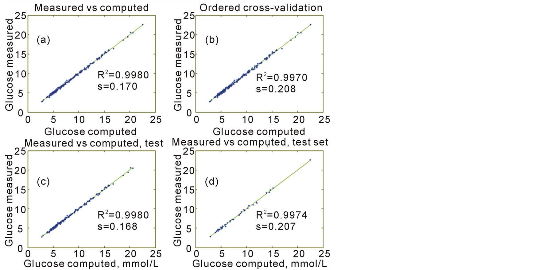
Figure 1. Scatter plots of measured versus computed glucose values.

Table 1. Results of PLS regression and Ridge regression.
there will be a low rank solution for X, which is equally good or better.
In conclusion, only dimension 12 should be used for the RR analysis. In this case there is no practical difference between PLS regression and RR. Full rank RR solution is also almost the same as the PLS one.
7.4. The Variance Var(b)
There is a common agreement that Var(b) is an important measure. Therefore, it is useful to look at how it increases by the number of dimensions used. This is shown in Figure 2. The trace function, tr, gives the sum of diagonal elements of a matrix. Thus, tr(Var(b)) is the sum of the variance of the regression coefficients. In a plot it is easier to use the square root to make the large values smaller, . For PLS regression it is

It is shown in Figure 2 for A = 1 to 50. At A = 12 the value is Std(b) = 2.8. In a full rank solution the value is Std(b) = 350. A high price is being paid, if full rank solution is chosen. It should be emphasized that Std(b)A is only a guidance measure. The variance of the regression coefficients can be derived by bootstrapping methods. But the values give guidance for what can be expected. Var(b) is slightly different for RR and the curve is lower (highest value is 115).
8. Variables and Latent Variables
Latent variables are estimates of the main axis in the hyper-ellipsoid, where data typically are located. Latent variables usually pick up the total variation much quicker than the variables. This is illustrated in Figure 3. The
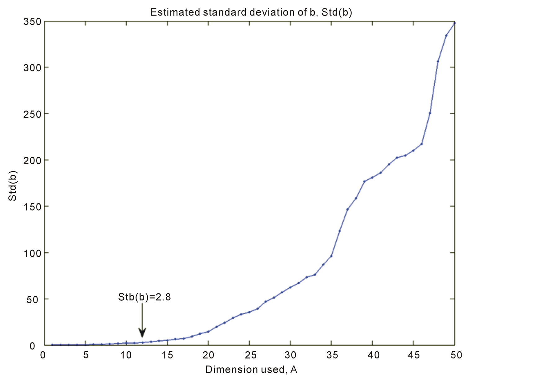
Figure 2.Plot of Std(b) versus dimension, A.
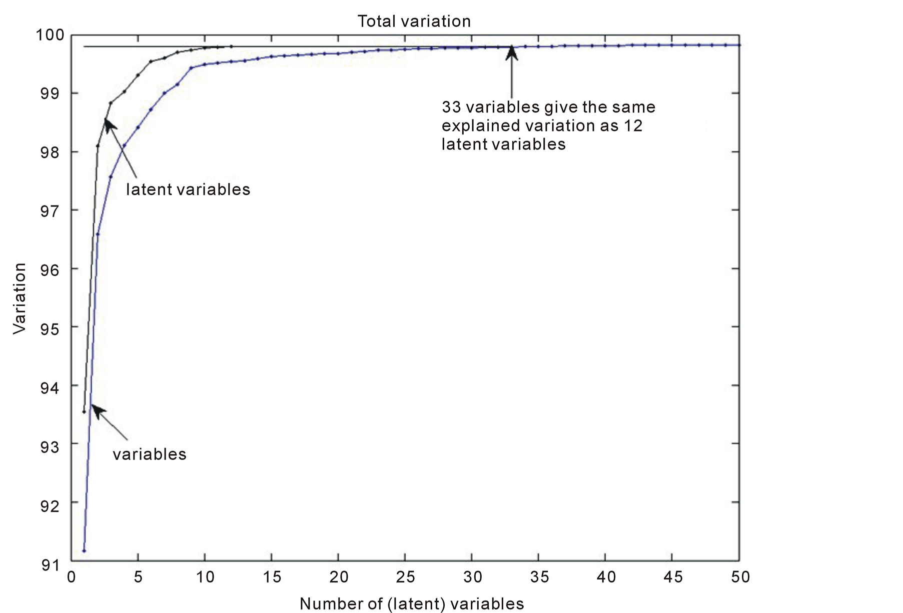
Figure 3. Explained variation, y-axis, versus the number of variables in the model, x-axis.
latent variables start at explained variation of 0.9354 and at the 12th the total variation has reached 0.9980. The variables start at 0.9069 and it is first at the 33th variable that the explained variation of 0.9980 is reached.
Mallows Cp theory is valid for regression analysis both for variables and latent variables. It states that, from a modelling point of view, it is important to keep the size of dimension as low as possible. Typically, the number is much smaller for latent structure regression than for regression methods based on variables.
Scientists/experimenters often tend to ask the question: Which variables are most important? When working with latent structure regression it is difficult to give a precise answer. For the FTIR data we can say that there are 1115 variables. Forward and backward analysis reduces this number to 50. Latent structure regression uses 12 dimensions in the regression analysis. All 50 variables contribute to the regression analysis. It is possible to explain the cumulative effects like at Figure 3.
9. Conclusions
A short review of standard regression analysis used in the popular program packages has been presented. It is pointed out that it is a serious problem in industry and applied sciences that the obtained results and presented in papers and reports may not be reliable.
A general framework is presented for linear regression, where the score vectors are orthogonal. Any set of weight vectors can be used that do not give score/loading vectors of zero size. Using the framework, different types of regression analysis can be tailored to different situations. The same type of graphic analysis can be carried out for any type of regression analysis within this framework; also when the start of the computations is variance and covariance matrices.
The algorithm can be viewed as an approximation to the full rank solution. Modelling stops, if further steps are not supported by data. Dimension measures, cross-validation and test sets are used to identify the dimension properly.
The H-principle is formulated in close analogy to the Heisenberg Uncertainty Inequality. It suggests that modelling should be carried out in steps, where at each step an optimal balance between the fit and associated precision should be obtained. A collection of methods, the H-methods, have been developed to implement the H-principle in different contexts.
H-methods have been applied for a number of years to different types of data within applied sciences and industry. The general experience is that they provide better predictions than other methods in the literature.
Acknowledgements
The Sime project is carried out in cooperation with Clinical Biochemistry, Holbæk Hospital, Denmark, on determining substances in blood plasma by FTIR spectroscopy. I appreciate the use of the results from the glucose analysis in the present article.
References
- Höskuldsson, A. (1996) Prediction Methods in Science and Technology. Vol. 1, Thor Publishing, Copenhagen.
- Höskuldsson, A. (2009) Modelling Procedures for Directed Network of Data Blocks. Chemometrics and Intelligent Laboratory Systems, 97, 3-10. http://dx.doi.org/10.1016/j.chemolab.2008.09.002
- Höskuldsson, A. (2008) H-Methods in Applied Sciences. Journal of Chemometrics, 22, 150-177. http://dx.doi.org/10.1002/cem.1131
- Höskuldsson, A. (1994) Data Analysis, Matrix Decompositions and Generalised Inverse. SIAM Journal on Scientific Computing, 15, 239-262. http://dx.doi.org/10.1137/0915018
- Clinical and Laboratory Standards Institute. http://www.clsi.org
- Kennard, R.W. and Stone, L.A. (1969) Computer Aided Design of Experiment. Technometrics, 11, 43-64. http://dx.doi.org/10.1080/00401706.1969.10490666
- Siotani, M., Hayakawa, T. and Fujikoshi, Y. (1985) Modern Multivariate Analysis: A Graduate Course and Handbook. American Science Press, Columbus.
- Roger, J.M., Palagos, B., Bertrand, D. and Fernandez-Ahumada, E. (2011) CovSel: Variable Selection for Highly Multivariate and Multi-Response Calibration. Application to IR Spectroscopy. Chemometrics and Intelligent Laboratory Systems, 106, 216-223. http://dx.doi.org/10.1016/j.chemolab.2010.10.003
- Höskuldsson, A. (2001) Variable and Subset Selection in PLS Regression. Chemometrics and Intelligent Laboratory Systems, 557, 23-38. http://dx.doi.org/10.1016/S0169-7439(00)00113-1
- Reinikainen, S.-P. and Höskuldsson, A. (2003) COVPROC Method: Strategy in Modeling Dynamic Systems. Journal of Chemometrics, 17, 130-139. http://dx.doi.org/10.1002/cem.770
- Grove, H., et al. (2008) Combination of Statistical Approaches for Analysis of 2-DE Data Gives Complementary Results. Proteome Research, 7, 5119-5124. http://dx.doi.org/10.1021/pr800424c
- McLeod, G., et al. (2009) A Comparison of Variate Pre-Selection Methods for Use in Partial Least Squares Regression: A Case Study on NIR Spectroscopy Applied to Monitoring Beer Fermentation. Journal of Food Engineering, 90, 300-307. http://dx.doi.org/10.1016/j.jfoodeng.2008.06.037
- Tapp, H.S., et al. (2012) Evaluation of Multiple Variate Methods from a Biological Perspective: A Nutrigenomics Case Study. Genes & Nutrition, 7, 387-397. http://dx.doi.org/10.1007/s12263-012-0288-4
- Bruker Optics, Germany. http://www.bruker.de
- Micro-Biolytics, Germany. http://www.micro-biolytics.de
- Perez-Guaita, D. et al. (2013) Modified Locally Weighted—Partial Least Squares Regression, Improving Clinical Predictions from Infrared Spectra of Human Serum Samples. Talanta, 170, 368-375. http://dx.doi.org/10.1016/j.talanta.2013.01.035