Applied Mathematics
Vol.5 No.2(2014), Article ID:42159,7 pages DOI:10.4236/am.2014.52025
An Automated Model for Fitting a Hemi-Ellipsoid and Calculating Eigenvalues Using Matrices
1College of Engineering, University of South Florida, Tampa, USA
2USF Health Morsani College of Medicine, University of South Florida, Tampa, USA
Email: aliciabillington@gmail.com, pfabri@health.usf.edu, wlee2@usf.edu
Received August 30, 2013; revised September 30, 2013; accepted October 7, 2013
ABSTRACT
Ellipsoid modeling is essential in a variety of fields, ranging from astronomy to medicine. Many response surfaces can be approximated by a hemi-ellipsoid, allowing estimation of shape, magnitude, and orientation via orthogonal vectors. If the shape of the ellipsoid under investigation changes over time, serial estimates of the orthogonal vectors allow time-sequence mapping of these complex response surfaces. We have developed a quantitative, analytic method that evaluates the dynamic changes of a hemi-ellipsoid over time that takes data points from a surface and transforms the data using a kernel function to matrix form. A least square analysis minimizes the difference between actual and calculated values and constructs the corresponding eigenvectors. With this method, it is possible to quantify the shape of a dynamic hemi-ellipsoid over time. Potential applications include modeling pressure surfaces in a variety of applications including medical.
Keywords:Modeling; Response Surfaces; Ellipsoid
1. Introduction
The Cartesian coordinate equation for an ellipsoid is given by the formula:
1) , where (h, j, k) represent the coordinates of the center of the ellipsoid and a, b, c represent the unit axis lengths from the center.
An alternate form of this equation is the matrix equation given by the formula:
2) , where
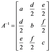 ,
, . This vector formulation provides size, shape, and orientation. The A matrix is assumed to be positive definite. Substitution gives the long form of the equation:
3) .
.
Here, the eigenvalues and eigenvectors of the A matrix give the corresponding squared length of the axis and the direction, respectively. Orthogonal eigenvectors are induced when the matrix is symmetric [1].
Previous papers have discussed using the method of least squares estimates (LSE) to converge on the ellipsoid best fit for a given set of data [2-5]. LSE analysis minimizes the sum of the distance (or squared difference) between the measured and predicted values of an ellipsoid. We have simplified this concept by implementing existing add-ins in Microsoft Excel such as Solver and Matrix.xla. Additionally, we have automated the process using VBA code so that as the hemi-ellipsoid alters shape and position we can continuously recalculate the new eigenvalues and eigenvectors of the ellipsoid.
Our goal was to create a program that automatically and continuously evaluates data from a pressure map for seated individuals. Currently, most medical institutions evaluate peak pressure when assessing patients for pressure build-up which can lead to pressure ulcer development. However, peak pressure is not the sole determinant in tissue breakdown [6]. Other studies have looked at using MRI and finite element analysis, but these studies do not use continuous data, are not over extended time periods, and involve significant expense [7-10]. The purpose of this analysis was to create a method that could show movement over time continuously and could be easily incorporated into existing care via a pressure map that many hospitals already own, without additional expenses.
2. Transformation and Least Squares Estimation
2.1. Calculated Values
In order to assess the validity of the method, we first tested the ability of the program to predict the values of a known ellipsoid. We chose the simple ellipsoid defined by the following equation: 
and considered only the superior half of the shape. We calculated the z values for x and y coordinates known to have corresponding values on the surface of the ellipsoid by solving for the unknown variable z:
 .
.
2.2 Predicted Values
The predicted values for z were calculated through minimization via quadratic optimization by gradient descent using the Solver Add-in in Microsoft Excel. Two models were created minimizing the absolute difference and the squared difference between z and![]() . The actual and predicted values from the model can be viewed in Table1 Multiple constraints were placed on the calculations. First, the equation for the matrix had to be satisfied (long form of equation above). Second, as previously mentioned, the
. The actual and predicted values from the model can be viewed in Table1 Multiple constraints were placed on the calculations. First, the equation for the matrix had to be satisfied (long form of equation above). Second, as previously mentioned, the  matrix must be made symmetric in order to assume orthogonal eigenvectors. Additional constraints on the
  matrix were made such that the matrix could be assumed positive definite. Finally, different lower bound values for
 ![]() were tested in order to allow Solver to find the optimal solution. We found that Solver was not always able to arrive at the best ellipsoid shape by simply allowing it to explore the surface on its own, but could converge if multiple values were tested. VBA code was written to create a loop to test various z
were tested in order to allow Solver to find the optimal solution. We found that Solver was not always able to arrive at the best ellipsoid shape by simply allowing it to explore the surface on its own, but could converge if multiple values were tested. VBA code was written to create a loop to test various z ![]() values and to select the value which minimized the sum of squared differences or the summed absolute difference. 3-D imaging of the selected predicted versus actual values are shown in Table2
values and to select the value which minimized the sum of squared differences or the summed absolute difference. 3-D imaging of the selected predicted versus actual values are shown in Table2

Table 1. Comparison of actual and predicted values of z using sum of least squares minimization with solver add-in in microsoft excel for a known ellipsoid.
Table 2. Images of hemi-ellipsoid taken with R excel add-in. Graphs 1 and 2 highlight the accuracy of the program on matching the actual (blue) and predicted (green) values. Graph 3 highlights the accuracy of correctly predicting the center (yellow).
The constraints are summarized here:
Objective Function:

Changing Cells:
![]()
 matrix h, j Constraints:


k = 0 the A matrix is assumed positive definite
3. Eigenvalue and Eigenvector Calculations
After the optimum predicted values were determined and thus the corresponding  matrix, the program was automated to select the
  matrix and calculate the associated eigenvalues and eigenvectors, as shown in Table3 The Jacobi Method in Matrix.XLA [11] was employed in order to ensure forced orthogonal vectors. Once the eigenvalues were determined, the square roots of the values were calculated to give the axis lengths of the ellipsoid.
4. Sample Data
After the validity of the program had been tested using a known ellipsoid, a 36 ´ 36 sample data set of measured values from a pressure map was analyzed. An ellipsoid shape was identified from the data automatically and assessed for characteristics of shape and size. The program was able to identify center values for the ellipsoid and eigenvalues that visually made sense, as shown in Figure 1. The calculated eigenvalues of 4.83, 8.38, and 71542.65 corresponded to x, y, and z-axes of 2.20, 2.90, and 267.47 respectively. Thus, we have illustrated that the program is capable of taking real data, locating an ellipsoid, and analyzing its shape.
5. Discussion
5.1. Analysis
Analysis of the data shows the strength of this program in accurately predicting the ellipsoid shape of the data.
Table 3. The calculated inverse A matrix with associated eigenvalues and eigenvectors. Note that the diagonal values of the inverse matrix are close to the actual values of 0.25 and that the distances calculated for the axis length of the ellipsoid are close to the actual value of 2 ´ 2 ´ 2 units.
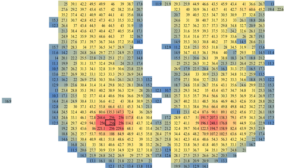
Figure 1. Sample data collected from a 36 ´ 36 matrix. Values increase in magnitude from blue to yellow to red. Box highlighted in black denotes cell which the program calculated as being at the center of the ellipsoid on left half of matrix.
Statistical analysis based on the 13 actual and predicted values of the known ellipsoid showed a very low average error of −0.288% and average absolute error of 0.507%. The center coordinates of the ellipsoid calculated automatically by the program were also extremely accurate, with an average −1.06% error. As discussed above, the  matrix gave values close to the expected value of 0.25, as seen in Table3 The summed difference between z and
 ![]() served as the optimization function in the Solver Add-in. The difference between the actual and predicted values was calculated to be only 0.266, again supporting the validity of this method in predicting the ellipsoid shape. The sum squared difference was also calculated, giving a value of 0.00019, with the above mentioned parameters also lower than with the summed difference. However, it was decided that the summed difference would be preferable to the sum squared difference as anticipated outliers will lead to distortion of the model. Finally, the square roots of the calculated eigenvalues reproduce close to the expected axis lengths of 2 units with only a 2.96% average absolute error.
served as the optimization function in the Solver Add-in. The difference between the actual and predicted values was calculated to be only 0.266, again supporting the validity of this method in predicting the ellipsoid shape. The sum squared difference was also calculated, giving a value of 0.00019, with the above mentioned parameters also lower than with the summed difference. However, it was decided that the summed difference would be preferable to the sum squared difference as anticipated outliers will lead to distortion of the model. Finally, the square roots of the calculated eigenvalues reproduce close to the expected axis lengths of 2 units with only a 2.96% average absolute error.
For the measured sample data set, the summed absolute difference between the measured and predicted values ranged from 364.52 to 1070.4 and the average absolute percent error was 20.478%. There are several considerations for the absolute percent error. First, the measured data is an irregular shape and is not a perfect hemi-ellipsoid. Second, while the overall shape may appear hemi-ellipsoid-like, outliers can affect the overall prediction of the model. We determined the values of the mound by eliminating low extreme values, but we did not eliminate high extreme values. Thus, it may be important in future applications to consider removal of these high peak values in order to focus on the values that best fit the shape of the hemi-ellipsoid.
Visualization of the data is an important validation method when testing modeling predictability, which allows interpretation of fit as well location of extreme differences and also verifies that the resulting model is actually ellipsoidal. The Add-in R Excel was used to give 3-D graphical representation, as shown in Figure 2 below. Additionally, Matlab was used to create a hemi-ellipsoid shape that fit the actual data based on using triangle-based cubic interpolation of the given values. A 3-D representation of the ellipsoid, actual, and predicted data are shown in Figure 3.
To our knowledge, this is the first description of the ischial tuberosities being modeled as hemi-ellipsoids using the matrix equation of an ellipsoid with sum of least squares in a continuous fashion. This model allows for continuous monitoring of data over long periods of sitting time due to its automation.
5.2. Limitations and Considerations
A major limitation of using a gradient descent method is that it is possible for local maxima or minima to be discovered that are not the true absolute maximum or minimum. In order to circumvent this, we created a loop allowed for different lower bound values for z to be assumed and it initiated the search in different points on the xy grid. We tuned the model to determine the best “center,” represented by a lower bound of “z”. Additionally, the assumption was made that the center of the ellipsoid was on the map. Thus, the parameter k was set equal to 0.
When automating, a trade-off has to be made between accuracy and computation time. Depending on the necessity for precision, a decreased stepping parameter may be desired to ensure the best possible fit occurs. The complexity of the problem and the running time for automation must be taken into consideration when deciding what step should be used and over what range of possible z lower bound values. For example, the running time from 0 to 150 with a step of 30 runs for 13.9 seconds while with a step of 15 runs for 38.8s. If multiple frames of data are collected per second over a period of several minutes to hours, the computation time increases to several hours.
A point of consideration when examining the results of the eigenvalues and eigenvectors is that Matrix.xla offered multiple means of calculating the eigen numbers. For example, the eigenvectors did not have to be assumed to be orthogonal with some methods. However, since we initially based our assumption of the  matrix as being positive definite, we chose the Jacobi method that forced orthogonalization. Ultimately, we felt that in order for the results to be comprehensible, it was most logical to force the vectors to be orthogonal.
The method described allows for complex modeling of 3-D data by assuming a hemi-ellipsoid shape. While some of the assumptions and constraints force that data to fit a symmetrical shape, it allows for a means of comparison between constantly evolving shapes. This method is useful in showing trends over time and has a variety of applications in modeling systems with changing hemi-ellipsoid-like shapes.
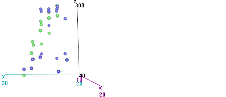

Figure 2. Sample data is in blue and predicted values are in green for the hemi-ellipsoid taken from the left portion of the matrix. The image on the left is a 3-D rendering of the data isolated as the mound from Figure 1. The image on the right models a different frame, and shows that the program can have difficulty in calculating the peak values at the top of the mound at times.
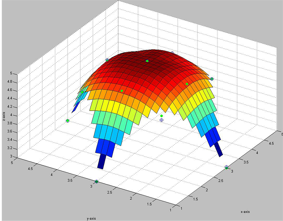
Figure 3. MATLAB rendering of ellipsoid created based on actual values of ellipsoid. Actual values are denoted by green circles. Predicted values are denoted by open blue circles with crosses.
Acknowledgements
A.B. would like to thank her faculty advisors and the Colleges of Engineering and Medicine at USF, as well as her patients, family, and Joshua M. Diggs.
REFERENCES
- S. B. Pope, “Algorithms for Ellipsoids,” Cornell University Report FDA 08-01, 2008.
- D. A. Turner, I. J. Anderson, J. C. Mason and M. G. Cox, “An Algorithm for Fitting an Ellipsoid to Data,” 1999. http://citeseerx.ist.psu.edu/viewdoc/summary?doi=10.1.1.36.2773
- E. S. Maini, “Enhanced Direct Least Square Fitting of Ellipses,” International Journal of Pattern Recognition and Artificial Intelligence, Vol. 20, No. 6, 2006, pp. 939-953. http://dx.doi.org/10.1142/S021800140600506X
- I. Markovsky, A. Kukush and S. Van Huffel, “Consistent Least Squares Fitting of Ellipsoids,” Numerische Mathematik, Vol. 98, No. 1, 2004, pp. 177-194. http://dx.doi.org/10.1007/s00211-004-0526-9
- S. J. Ahn, “Least Squares Orthogonal Distance Fitting of Curves and Surfaces in Space,” Ph.D. Dissertation, University of Stuttgard Stuttgard, 2004.
- A. Gefen, “Reswick and Rogers Pressure-Time Curve for Pressure Ulcer Risk. Part 1,” Nursing Standard, Vol. 23, No. 45, 2009, pp. 64-74. http://dx.doi.org/10.7748/ns2009.07.23.45.64.c7115
- S. Portnoy, N. Vuillerme, Y. Payan and A. Gefen, “Clinically Oriented Real-Time Monitoring of the Individual’s Risk for Deep Tissue Injury,” Medical & Biological Engineering & Computing, Vol. 49, No. 4, 2011, pp. 473-483.
- L. Agam and A. Gefen, “Toward Real-Time Detection of Deep Tissue Injury Risk in Wheelchair Users Using Hertz Contact Theory,” Journal of Rehabilitation Research and Development, Vol. 45, No. 4, 2008, pp. 537-550. http://dx.doi.org/10.1682/JRRD.2007.07.0114
- A. Gefen, “Bioengineering Models of Deep Tissue Injury,” Advances in Skin and Woundcare, Vol. 21, No. 1, 2008, pp. 30-36. http://dx.doi.org/10.1097/01.ASW.0000305403.89737.6c
- E. L. Ganz, N. Shabshin, Y. Itzchak and A. Gefen, “Assessment of Mechanical Conditions in Sub-Dermal Tissues during Sitting: A Combined Experimental-MRI and Finite Element Approach,” Journal of Biomechanics, Vol. 40, No. 7, 2007, pp. 1443- 1454. http://dx.doi.org/10.1016/j.jbiomech.2006.06.020
- “Matrices and Linear Algebra,” Reference Guide for Matrix.xla, 2006. http://digidownload.libero.it/foxes/matrix/MatrixTutorial1.pdf