Applied Mathematics
Vol.5 No.8(2014), Article ID:45614,13 pages DOI:10.4236/am.2014.58105
Finite Element Solution of a Problem for Gravity Gyroscopic Equation in the Time Domain
Mikhail Nikolayevich Moskalkov¹, Dauletbay Utebaev²
1National Aviation University, Kyiv, Ukraine
2Berdakh Kara-Kalpak State University, Nukus, Uzbekistan
Email: moskalkov@hotmail.com, dutebaev_56@mail.ru
Copyright © 2014 by authors and Scientific Research Publishing Inc.
This work is licensed under the Creative Commons Attribution International License (CC BY).
http://creativecommons.org/licenses/by/4.0/


Received 2 March 2014; revised 2 April 2014; accepted 9 April 2014
ABSTRACT
To solve the equation for gravity-gyroscopic waves in a rectangular domain, the distinguished algorithm for the solution of the Cauchy problem for a second-order transient equation is proposed. This algorithm is developed by using the time-varying finite element method. The space derivatives in the gravity-gyroscopic wave equation are approximated with finite differences. The stability and accuracy of the method are estimated. The procedure for the implementation of the method is developed. The calculations were performed for determining the steady-state modes of fluctuations of the solutions of the gravity-gyroscopic wave equation depending on the problem parameters.
Keywords:Finite Element Method, Difference Scheme, Error Estimate, Gravity-Gyroscopic Waves

1. Introduction
The strengthening of requirements for solving complex problems in scientific and technological researches results in the improvement of existing numerical computation algorithms. This improvement is of particular importance in studying complex nonstationary processes, for example, the propagation of gravity-gyroscopic waves.
The mathematical statement of problems in the theory of internal waves, including gravity-gyroscopic waves, and methods for solving such problems are discussed in publications [1] -[6] . In publications [1] -[3] , the equations for describing the propagation of internal waves are derived using the Bussinesk approximation. Various analytical methods of solving problems in the linear theory of gravity-gyroscopic waves are proposed in publications [3] -[6] . Specifically, in publications [4] [5] , the modes of steady-state oscillations associated with gravity-gyroscopic waves are defined depending on the coefficients of equations describing the propagation of gravity-gyroscopic waves in response to a harmonic disturbance in the unbounded medium.
Since analytical methods not always allow solutions of problems for arbitrary data and solution regions to be obtained, numerical methods are used. In solving nonstationary problems, semidiscrete methods are used, that is, the methods with initial approximation only for spatial variables followed by the solution of the Cauchy problem by using finite-difference algorithms. These methods provide an order of accuracy not higher than the second one [7] [8] .
To enhance the calculation accuracy, it is necessary to use numerical algorithms providing a higher order of accuracy [9] . This is possible due to the finite element method. Among numerous publications for the finite element method, we refer to publications [10] -[12] which specify the methods and algorithms for solving stationary and nonstationary problems in the mathematical physics. In publication [13] , an algorithm for solving second-order nonstationary equations, which provides the fourth order of accuracy, is proposed. According to publications [14] -[18] , this algorithm was used and substantiated in solving various problems in the mathematical physics which are described by equations for oscillations. The methods for the implementation of this algorithm were developed, as well as the stability and convergence of the algorithm in the classes of Soboliev functions were proved.
2. Problem Statement
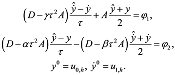
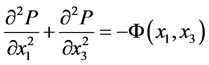
Consider the following problem:
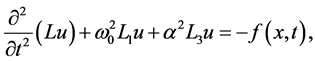 (1)
(1)
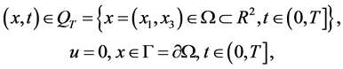 (2)
(2)
 , (3)
, (3)
where , and
, and .
.
Equation (1) is obtained from the set of hydrodynamic equations in Boussinesq approximation [1] -[5] . This equation describes small oscillations of stratified fluid with density  and
and  being twice the speed of fluid rotation around
  axis. The quantity
 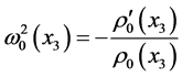 denotes the square of the Brent-Väisälä frequency. The fluid velocity is calculated using the formula
 . We will also assume that the Brent-Väisälä frequency
  is constant. Equation (1) is not classical and belongs to the Sobolev equations of composite type [1] -[3] .
Let us define the generalized solution of problem (1)-(3) as a function , that has a derivative
  for each
  and satisfies the following relationships for
  [1] :
[1] :
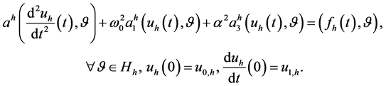
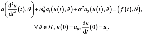 (4)
(4)
where
 ,
,  and
and  is a function of abstract argument
  with values in H. The issues of the solution existence and its properties were discussed in the works [1] -[3] .
3. Spatial and Time Approximation
Let us construct a subspace  that approximates H. Let us also introduce a mesh
 , where
 ,
,
 . In this case
  -is a space of mesh functions
  with the norm
 where constant M is independent of
  [7] .
[7] .
With the use of the corresponding quadrature formulae , we approximate
  on the mesh and derive an approximated mesh solution from Equation (4):
 (5)
(5)
The problem defined by Equation (5) corresponds to the following Cauchy problem for the function :
:
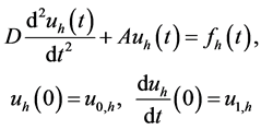 (6)
(6)
where
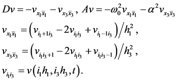 (7)
(7)
Also
 (8)
(8)
where ,
, ![]() is a projection operator
is a projection operator  and
and . Difference operators D, A approximate differential operators
  and
and  with a second order error.
Now let us consider a discretization of the Cauchy problem for the time variable (6). Let  be a mesh on the time segment
  (for simplicity we assume the uniform mesh). From equation (6) the following identity can be deduced for each segment
 :
:
 (9)
(9)
Let us seek an approximate solution of problem (6) in the form of the Hermitian spline of the third order similarly to [10] [11] :
![]() where
where

![]()
![]()

 .
.
Selecting the various weight functions , namely:


and choosing the parameters , the following two parameter vector difference scheme can be obtained from Equation (9) [13] [14] :
 (10)
(10)
where
 ,
,  ,
, 
The parameters  are subject to the fourth order approximation condition for Scheme (10) [14] .
 . (11)
For definiteness, assume the following values of parameters, .
.
4. Scheme Implementation Algorithm
For implementation of Scheme (10), it is necessary to solve the system of two equations with respect to unknown variables :
:
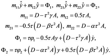 (12)
(12)
Let us assume that condition (11) holds. Excluding  from Equations (12) we obtain an equation to find
 :
:
 (13)
(13)
where
![]()

The first algorithm of implementation of Scheme (12) is a direct solving Equation (13) with further calculation of  from the first equation in System (12):
 .
.
The second algorithm of implementation of Scheme (12) is reduced to solving the following two equations [13] [14] for each time increment:

where 
![]()
The matrix C can be factorized: , where
  are the roots of the equation
![]() .
.
For instance, if , we have
 .
.
Then

 .
.
For inversion of the matrices  the direct square root method was used once at the initial time. For all other layers the solutions were obtained by multiplying the matrix
  by vectors
 .
.
5. Stability and Convergence
Theorem 1. [13] [14] . If 
 and
and ,
,
![]() (14)
(14)
then the solution  of scheme (10) converges to the solution of Problem (5)
 ![]() and the following estimate holds:
and the following estimate holds:
 .
.
The proof of the statement is based on the separate transformation of two layer scheme (10) to a three layer scheme for both solution y and its derivative . Condition (14) for the chosen values of the parameters (
 ,
, and the corresponding value
 ) gives the following restriction on the time increment:
 . (15)
For evaluation of the accuracy of Scheme (10) the error  shall be estimated. Applying the procedure used in the theory of finite difference schemes for such estimates [8] the final result can be formulated.
Theorem 2. If stability condition (15) of Scheme (10) holds the solution  converges to a sufficiently smooth solution of Problem (1)-(3) and the following estimate holds:
 .
.
6. Computational Experiments
Let us proceed to the description of the computational experiment. The asymptotic amplitude problem for the solution of Equation (1) under the uniform initial conditions on the plane
 was studied in the works [2] [3] . As a source of excitation the oscillations in the vicinity of a thin plate of 2 in length inclined at angle
 ![]() with
with  axis were assumed. The law of plate oscillations as a rigid body immersed in a liquid is as follows:
 , where
  and with
 .
.
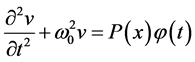
It has been proven that the asymptotic amplitude  exists and satisfies the equation
 . (16)
When  and
and  Equation (16) is an elliptic one. Under the condition of
 , Equation (16) is of the hyperbolic type. It means that there are differences in the behavior of the solution
  in its way to the steady state. Furthermore, it has been shown that when
 the solution decays according the following law
 .
.
Let us consider the right-hand member of Equation (1) as an excitation factor of the fluid motion that is acting on a small segment of  in length which is small compared to the overall length of the domain:
 ,
,

and during the finite period of time:

The initial conditions are uniform:
 .
.
The dimensions of the domain are ,
,  and
and![]() . The mesh parameters are as follows:
. The mesh parameters are as follows: ,
,  ,
,![]() .
.
The results of the simulations are shown in Figures 1-16. For all simulations the frequency of induced oscillations is .
.
For the equation parameters  and
and  such values were used at which the type of Equation (16) was elliptic or hyperbolic or singular due to fulfillment of the following equalities: either
 , or
, or .
.
The plot of the time variation of the amplitude  at the point
  is shown in Figure 1. The plot shows that the time of the external influence on the medium is limited by the segment
 ![]() for all alternative simulations.
for all alternative simulations.
The simulation plots for five different combinations of the parameters  that have resulted in the interesting solutions with a typical behavior (as follows from the results not included in this work) are shown below. Let us introduce the parameter
 .
.
For the first case 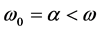 and so
 . This result is trivial in a certain sense. In this case, Equation (1) can be written as an ordinary differential equation:
 where
where  is the solution of the Dirichlet problem for the Poisson elliptic equation:
 .
.
Figure 2 shows the plot of the amplitude oscillations at the middle point of the domain![]() , i.e. at
, i.e. at ,
,  for the values
 .
.
Figure 3 and Figure 4 show the simulation plots for two instants of time with the positive and negative solution values.
The next plots (Figures 5-7) show the solutions for a hyperbolic case (the problem parameters are described in the caption of Figure 5).
Let us consider an elliptic case, noting that  (Figures 8-10).
The following results correspond to the singular cases with  (Figures 11-13) and
  (Figures 14-16).
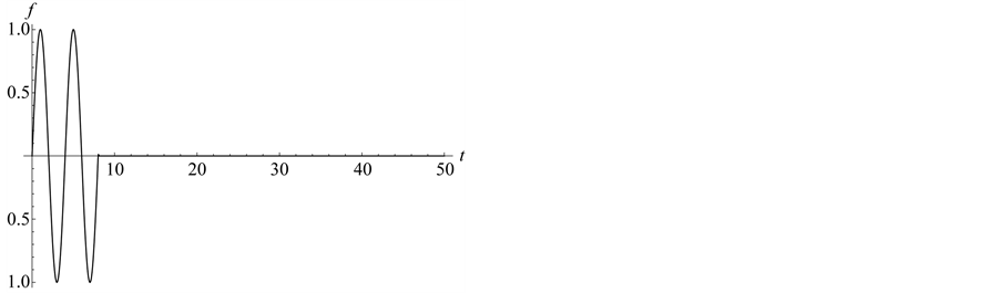
Figure 1. Function .
.
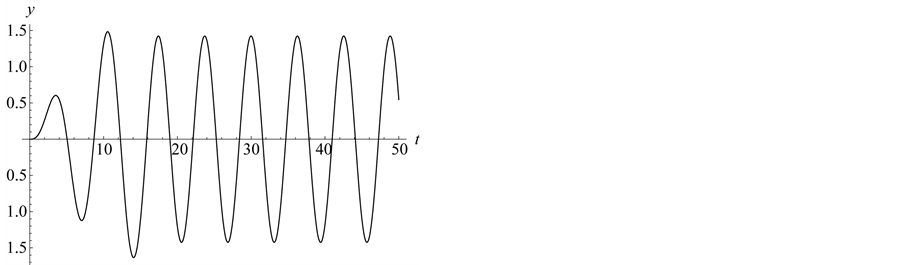
Figure 2. Function ,
,  , ω = 1.57080,
  ,
, .
.
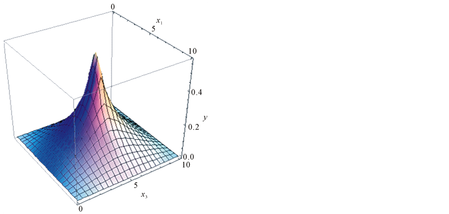
Figure 3. Solution  for
for![]() .
.
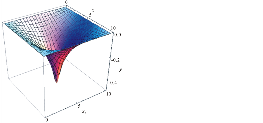
Figure 4. Solution  for
for![]() .
.
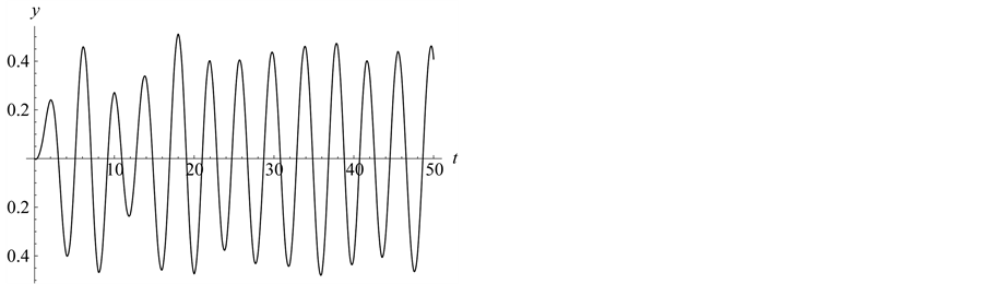
Figure 5. Function ,
,  , ω = 1.57080,
  ,
, .
.
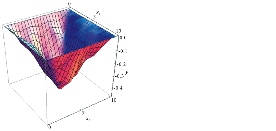
Figure 6. Solution  for
for![]() .
.
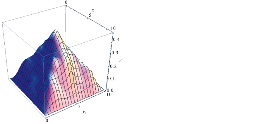
Figure 7. Solution  for
for![]() .
.
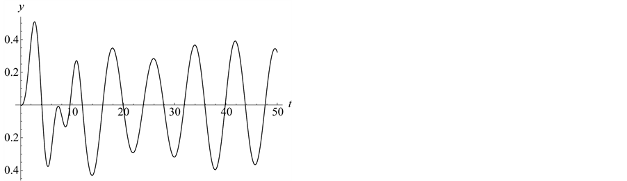
Figure 8. Function ,
,  , ω = 1.57080,
 ![]() ,
, .
.
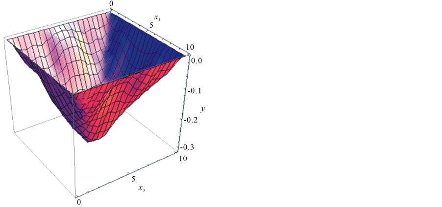
Figure 9. Solution  for
for![]() .
.
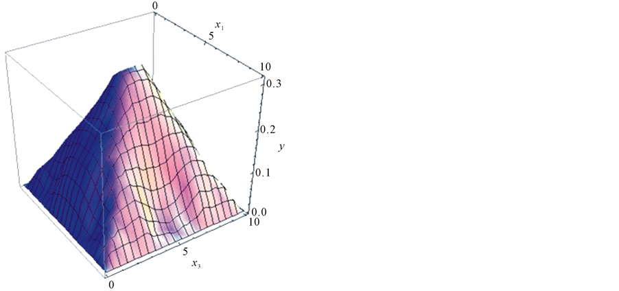
Figure 10. Solution  for
for![]() .
.
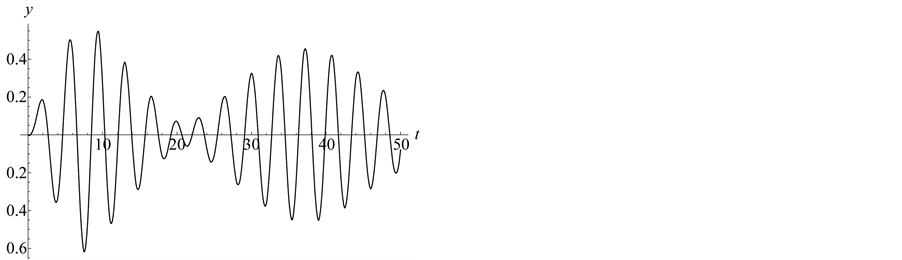
Figure 11. Function ,
,  , ω = 1.57080,
 ![]() ,
, .
.
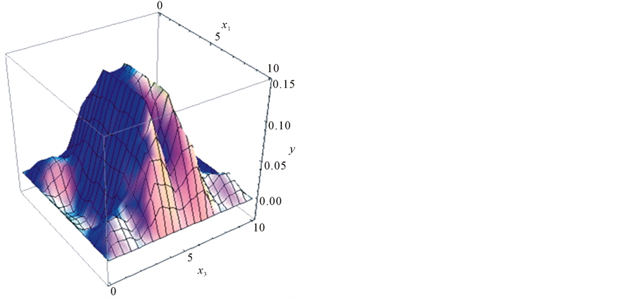
Figure 12. Solution  for
for![]() .
.
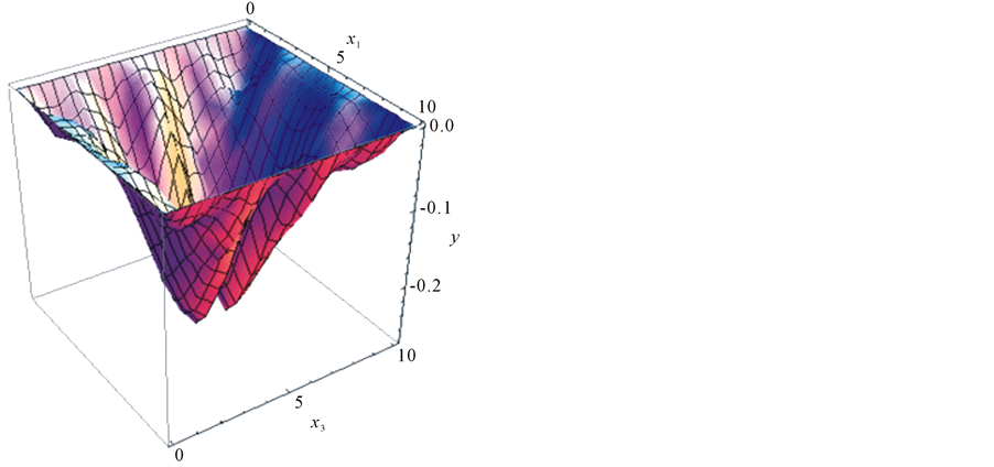
Figure 13. Solution  for
for![]() .
.
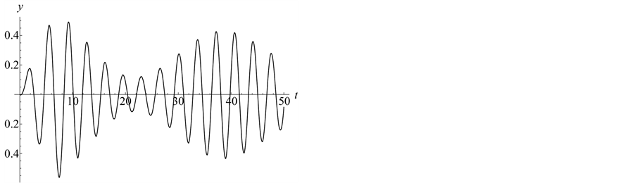
Figure 14. Function ,
,  ,
, ![]() ,
, ![]() ,
, .
.
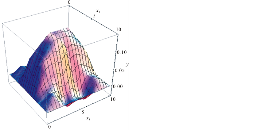
Figure 15. Solution  for
for![]() .
.
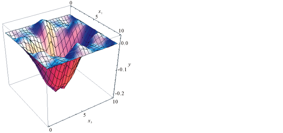
Figure 16. Solution  for
for![]() .
.
7. Conclusions
The following conclusions can be drawn on the basis of the comparative analysis of the simulation results:
• for all parameter combinations the solution achieves a steady state regime (Figures 3-16);
• there are no significant differences between the parameter sets of hyperbolic or elliptic types (Figure 6, Figure 7 and Figure 9, Figure 10): in both cases the form of the solution form is determined by the shape of spatial domain;
• the singular cases show that the steady state regime corresponds to equation of asymptotic amplitude (14): the solution shown in Figure 12, Figure 13 is “stretched” along ox1 axis in the middle region and corresponds to the asymptotic equation ; similarly in Figure 15, Figure 16 the solution is “stretched” along the ox3 axis and corresponds to the limiting equation,
 ;
;
• for  no decay of the solution amplitude
  is observed.
The last observation can be explained as follows. For the solution of problem (1)-(3) the following law of energy conservation holds:
 this conservation law can be obtained from identity (4) by simple manipulations assuming
![]() . The same conservation law holds for the Cauchy problem solution of Equation (1) in the entire plane
. The same conservation law holds for the Cauchy problem solution of Equation (1) in the entire plane . However, along the entire plane the energy has no constraints in the form of the domain boundaries thus it is dissipated along the infinite plane
  leading to the following behavior of the solution as a function of t, as was shown in [3] :
 .
.
References
- Whitham, G.B. (1974) Linear and Nonlinear Waves. Wiley, Hoboken.
- Miropolsky, Y.Z. (1981) Dynamics of Internal-Waves in the Ocean. Gidrometeoizdates, Moscow.
- Gabov, S.A. and Sveshnikov, A.G. (1990) Linear Problems in the Theory of Non-Steady-State Internal Waves. Nauka, Moskow.
- Gabov, S.A. and Pletner, Y.D. (1985) A Nachal-No-Kraevoy Problem for the Gravity-Gyros-Copic Waves. Journal of Computational Mathematics and Mathematical Physics, 25, 1689-1696.
- Gabov, S.A. and Pletner, Y.D. (1987) The Gravity-Gyroscopic Waves: The Angular Potential and Its Application. Journal of Computational Mathematics and Mathematical Physics, 27, 102-113.
- Iskendarov, B.A., Mamedov, J.Y. and Sulaimanov, S.E. (2009) Mixed Problem for the Gravity-Gyroscopic Waves in the Boussinesq Approximation in an Infinite Cylindrical Domain. Journal of Computa-tional Mathematics and Mathematical Physics, 49, 1659-1675.
- Samarskii, A.A. (1977) Theory of Difference Schemes. Nauka, Moskow.
- Samarskii, A.A. and Vabishchevich, P.N. (2007) Additive Difference Schemes for Problems in Mathematical Physics. URSS, LCI, Moscow.
- Moskalkov, M.N. (1975) On a Property of Schemes of High Order for One-Dimensional Wave Equation. Journal of Computational Mathematics and Mathematical Physics, 15, 254-260.
- Zienkiewicz, O.C. (1971) The Finite Element Method in Engineering Science. McGraw-Hill, London.
- Zienkiewicz, O.C. and Morgan, K. (1983) Finite Elements and Approximation. Wiley, Hoboken.
- Zienkiewicz, O.C. and Taylor, R.L. (2000) The Finite Element Method. Butterworth-Heinemann.
- Moskalkov, M.N. (1980) Scheme of the High-Accuracy Finite Element Method for Solving Non-Steady-State SecondOrder Equations. Differential Equations, 16, 1283-1292.
- Moskalkov, M.N. and Utebaev, D. (2005) Investigation of Difference Schemes of Finite Element Method for Second-Order Unsteady-State Equations. Journal Computation and Applied Mathematics, Kiev, No. 92, 70-76.
- Moskalkov, M.N. and Utebaev, D. (2012) Comparison of Some Methods for Solving the Internal Wave Propagation Problem in a Weakly Stratified Fluid. Mathematical Models and Computer Simulations, 3, 264-271. http://dx.doi.org/10.1134/S2070048211020086
- Moskalkov, M.N. and Utebaev, D. (2010) Finite Element Method for the Gravity-Gyroscopic Wave Equation. Journal Computation and Applied Mathematics, 2, 97-104.
- Moskalkov, M.N. and Utebaev, D. (2011) Convergence of the Finite Element Scheme for the Equation of Internal Waves. Cybernetics and Systems Analysis, 47, 459-465. http://dx.doi.org/10.1007/s10559-011-9327-1
- Moskalkov, M.N. and Utebaev, D. (2009) The Convergence of Finite Element Method for a Hyperbolic Equation with Generalized Solutions. Uzbek Mathematical Journal, Uzbekistan, No. 2, 119-128.