Applied Mathematics
Vol.4 No.5A(2013), Article ID:31573,11 pages DOI:10.4236/am.2013.45A003
High-Order Spectral Stochastic Finite Element Analysis of Stochastic Elliptical Partial Differential Equations
1Department of Accounting and Information System, Chang-Jung Christian University, Gueiren, Tainan, Taiwan 2Department of Civil Engineering, Feng-Chia University, Taichung, Taiwan
Email: xsheu@hotmail.com
Copyright © 2013 Guang Yih Sheu. This is an open access article distributed under the Creative Commons Attribution License, which permits unrestricted use, distribution, and reproduction in any medium, provided the original work is properly cited.
Received February 27, 2013; revised April 23, 2013; accepted April 30, 2013
Keywords: Spectral Stochastic Finite Element Method; Generalized Polynomial Chaos Expansion; High-Order Elements
ABSTRACT
This study presents an experiment of improving the performance of spectral stochastic finite element method using high-order elements. This experiment is implemented through a two-dimensional spectral stochastic finite element formulation of an elliptic partial differential equation having stochastic coefficients. Deriving this spectral stochastic finite element formulation couples a two-dimensional deterministic finite element formulation of an elliptic partial differential equation with generalized polynomial chaos expansions of stochastic coefficients. Further inspection of the performance of resulting spectral stochastic finite element formulation with adopting linear and quadratic (9-node or 8-node) quadrilateral elements finds that more accurate standard deviations of unknowns are surprisingly predicted using quadratic quadrilateral elements, especially under high autocorrelation function values of stochastic coefficients. In addition, creating spectral stochastic finite element results using quadratic quadrilateral elements is not unacceptably time-consuming. Therefore, this study concludes that adopting high-order elements can be a lower-cost method to improve the performance of spectral stochastic finite element method.
1. Introduction
A stochastic partial differential equation is a partial differential equation having stochastic coefficients or forcing terms. Problems expressed as stochastic partial differential equations include such as population dynamics and elastostatics with the uncertainty in the spatial variability of mechanical properties. The spectral stochastic finite element method [1] may be the most popular numerical tools for solving stochastic partial differential equation. Briefly, deriving a spectral stochastic finite element formulation couples a deterministic finite element formulation and representations of those stochastic coefficients and forcing terms. These representations of stochastic forcing terms and coefficients are derived by such as generalized polynomial chaos [2] and Karhunen-Lo- ève expansions [3].
Numerous spectral stochastic finite element formulations are available for some branches of science and engineering. References [4,5] are two recent examples. Nevertheless, the performance of spectral stochastic finite element method is not always satisfactory. For example, the spectral stochastic finite element method predicts less accurate mean values or standard deviations of random fields than the spectral stochastic meshless local Petrov-Galerkin method does [6]. Similar experiences bring about the motive for improving the performance of spectral stochastic finite element method.
Since a spectral stochastic finite element formulation contains a deterministic finite element solution and random field representations, improving the performance of spectral stochastic finite element method may be through adopting more accurate deterministic finite element formulation or random field representations. Available studies (e.g. [1]), which were devoted to evaluate the performance of spectral stochastic finite element method, seem to focus on the latter method. Experiences of applying a spectral stochastic finite element formulation using high-order elements seem to be unavailable. After a web search, only Ngah and Young (2007) [7] had adopted quadratic quadrilateral elements to predict the performance of composite structures. Thus, this study focuses on applying the spectral stochastic finite element method using high-order elements and evaluating the accuracy of corresponding spectral stochastic finite element results. A two-dimensional elliptical partial differential equation having stochastic coefficients is chosen as the model problem. A spectral stochastic finite element formulation of such a stochastic partial differential equation is derived by coupling a two-dimensional deterministic finite element formulation of an elliptical partial differential equation with generalized polynomial chaos expansions of stochastic coefficients. Two benchmark problems having deterministic analytical solutions are then introduced to test the performance of resulting spectral stochastic finite element formulation with adopting linear and high-order finite elements.
The remainder of this study is organized in three sections. Section 2 presents the two-dimensional spectral stochastic finite element formulation of an elliptical partial differential equation having stochastic coefficients. Section 3 evaluates the performance of resulting spectral stochastic finite element formulation. Based on this performance evaluation, Section 4 draws some conclusion.
2. Spectral Stochastic Finite Element Formulation
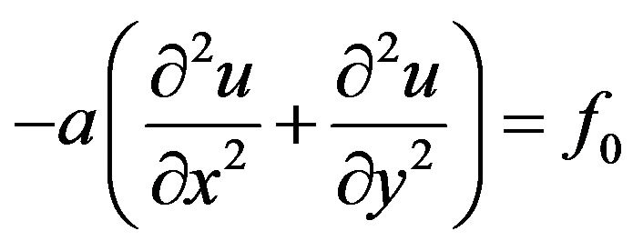
Suppose x and y are the spatial coordinates, q is an event in the probability space, W is a problem domain, and G is its boundary. The model problem of this study is described by
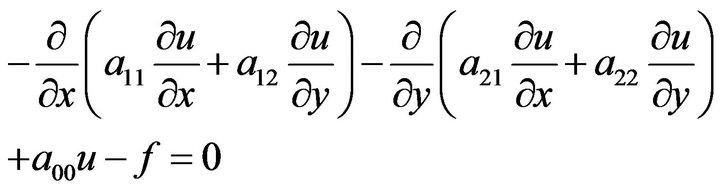 (1)
(1)
where u is the unknown (such as temperature and stream function),  and f are coefficients. In addition, the unknown u, coefficients
 , and f are dependent upon x, y, and q. Meanwhile, boundary conditions are
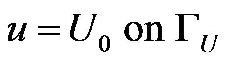 (2a)
(2a)
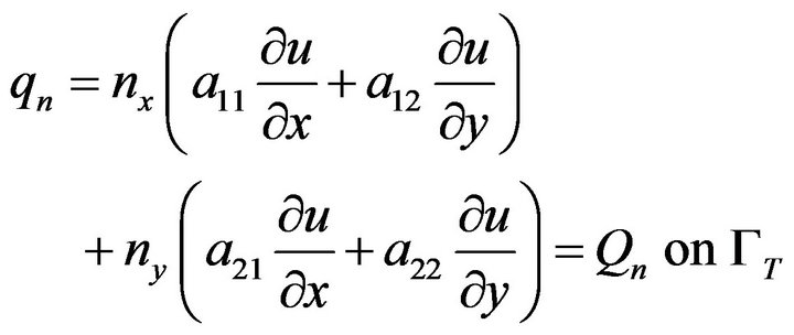 (2b)
(2b)
in which  and
and  are two known functions,
  is the essential boundary, GT is the natural boundary, qn is the secondary variable, nx and ny are the components of a unit vector n normal to GT, and
To derive a spectral stochastic finite element formulation of (1), a two-dimensional deterministic finite element formulation of an elliptical partial differential equation is needed. Suppose w is the test function. The weak form of (1) is
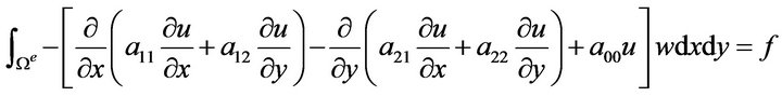 (3)
(3)
where the superscript e denotes an element. Simplifying (3) by the divergence theorem yields
 (4)
(4)
where Ge is the boundary of We, and ds is the arc length of an infinitesimal line along the boundary Ge. Next, approximate u over each We by
 (5)
(5)
in which N is the total number of nodes in each We, and y is the shape function. Substituting (5) into (4) and setting  yield
yield
 (6)
(6)
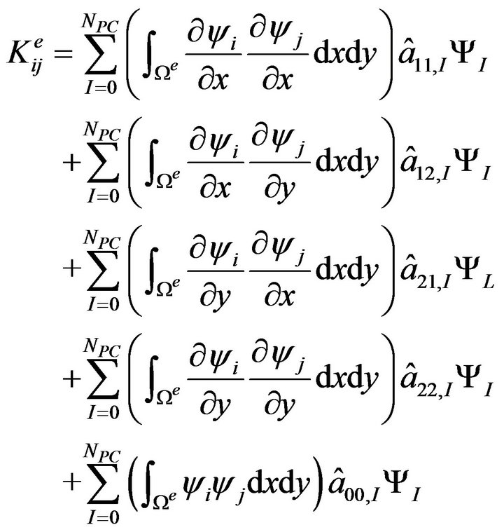
Equation (6) can be summarized in the form as
 (7)
(7)
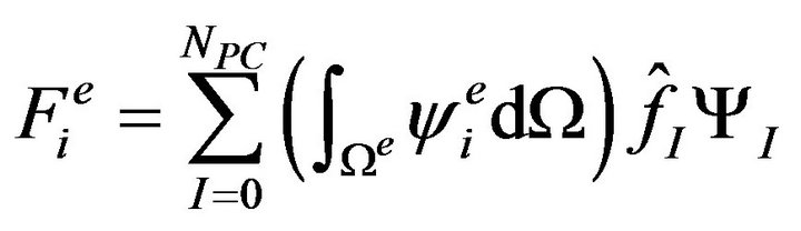
where
 (8a)
(8a)
 and
and  (8b)
(8b)
Moreover, (7) can be written more succinctly in matrix algebra as
 (9)
(9)
in which  contain all the nodal u value in each We. Repeatedly deriving (9) for all We and assembling all the resulting expressions based on a global numbering system yield
 (10)
(10)
in which NT is the total number of nodes in the problem domain W. Since  and f are dependent upon x, y, and q, (10) is not ready for use. The generalized polynomial chaos expansion is chosen to estimate the distribution of
  and f. Similar manipulating the published study [6], generalized polynomial chaos expansions of
  and f are defined by
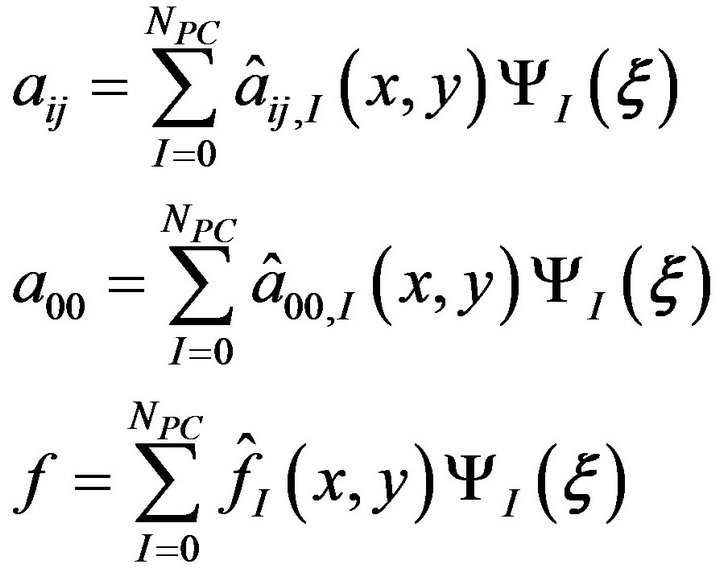 (11)
(11)
where ,
,  represent the multivariate orthogonal polynomial of
 ,
,  denote multi-dimensional uncorrelated random variables having zero mean and unit variance (for facilitating the computation of mean values and standard deviations of
  and f), NPC is equal to
 , P is the highest order of Ψ, and n is the total number of uncorrelated random variables.
For facilitating the computation of (11), Ψ0,
 ,
,  and
and  are; respectively, set to 1, mean values of aij, a00 and f; respectively. Furthermore, computing coefficients
  and
and  needs the orthogonal relationship,
in which  is the ensemble average. For example,
  are computed by
 (12)
(12)
in which  is computed as follows: If f and g are two functions,
  is computed by 1) Continuous case:
 (13a)
(13a)
2) Discrete case:
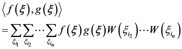 (13b)
(13b)
where  are the weighting functions. In (1), the succeeding study focuses on the continuous random fields; therefore, Table 1 [6] lists examples of orthogonal polynomials, statistical distributions and weighting functions to generate
 , and
, and ; respectively.
Substituting (11) into (8a) yields
 (14)
(14)
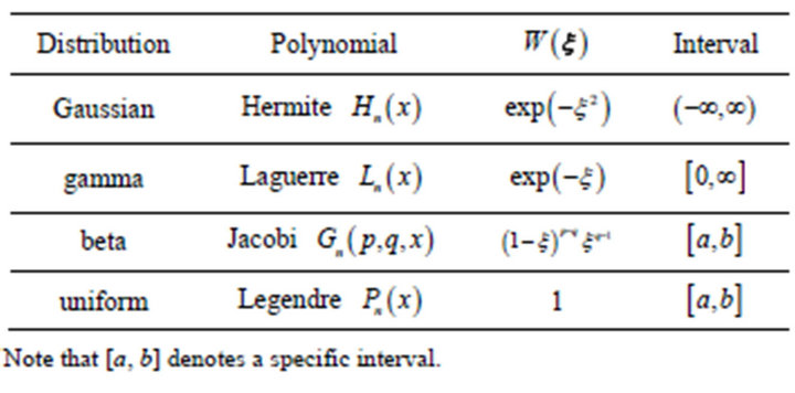
Table 1. Examples of polynomials and corresponding weighting functions and statistical distributions for generating the generalized polynomial chaos [6].
Similarly, substituting (11) into (8b) yields
 (15)
(15)
Meanwhile, the generalized polynomial chaos expansion of u is
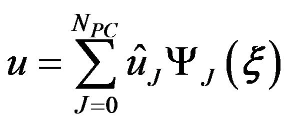 (16)
(16)
Modifying (10) with (14) and (16) results in
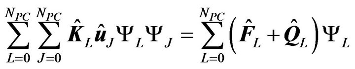 (17)
(17)
Requiring the residual resulting from a finite representation of u (i.e. truncating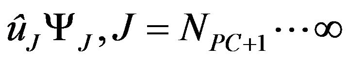 ) to be orthogonal to the approximation space spanned by
  yields
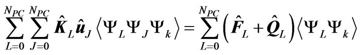 (18)
(18)
Solving (18) can obtain . Accumulating the resulting
  values can construct the generalized polynomial chaos expansion of u.
3. Results and Discussions
Two benchmark problems are introduced to evaluate the performance of (18) with adopting linear and high-order elements. The first benchmark problem involves a heat conduction problem over a square region. The second problem involves the transverse deflection of a square membrane.
3.1. Heat Conduction over a Square Region
As outlined by Figure 1, suppose a heat conduction problem over a unit square region in where Ñ is the gradient vector. The origin of x and y coordinates locates at the lower left corner. The boundaries  and
and  are insulated. The other boundaries
  and
and  are maintained at zero temperature. In addition, the square region is subjected to a uniform heat generation.
To predict the temperature T, the governing equation is
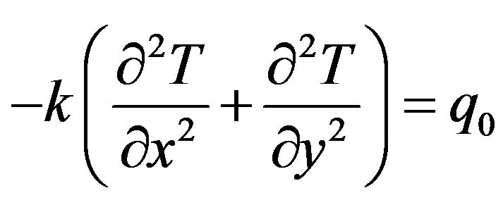 (19)
(19)
where k is the thermal conductivity and  is the rate of uniform heat generation. In addition, the boundary conditions are
 (20)
(20)
Similarly manipulating (7), the deterministic finite element formulation of (19) is
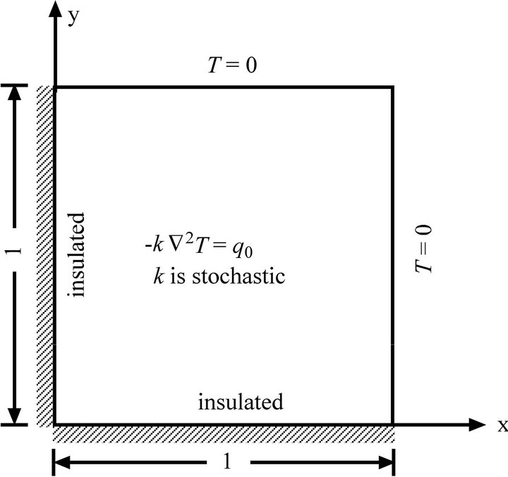
Figure 1. A heat conduction problem over a square region (not to scale).
 (21)
(21)
where
 (22)
(22)
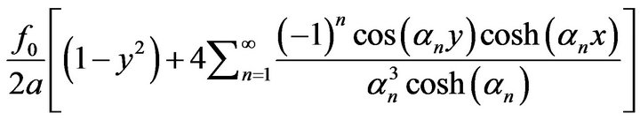
Moreover, if the coefficient k is deterministic, the analytical solution of (19) is [8]
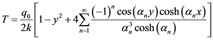 (23)
(23)
where  . However, the succeeding study considers that the thermal conductivity k is stochastic. Assume the distribution of k is described by
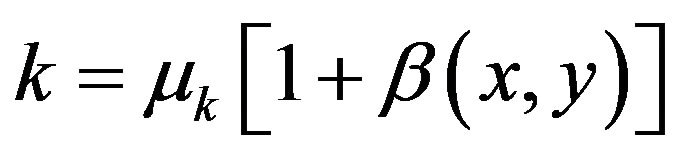 (24)
(24)
where  is the mean value of k and this
  value is independent upon x and y. Meanwhile,
  is a zero-mean, scalar, homogeneous random field with its autocorrelation function Gb equal to
 (25)
(25)
where d1 and d2 denote the correlation lengths, Sk is the standard deviation of thermal conductivity  and
and  represent two points of the square region.
To compare the predicted temperature T with adopting linear or high-order elements, essential data is provided below 1) Define the problem domain W as  and
and .
.
2) Generate two cases of the finite element discretizations. As outlined by Figure 2, the left sub-figure denotes the first case which is composed of 25 nodes and 16 linear quadrilateral elements. The right sub-figure denotes the second case which is composed of 81 nodes and 16 quadratic (9-node) quadrilateral elements.
3) Consulting with Table 1 and the previous study [6], experiment to represent k by the Lauguerre polynomial chaos. If the accuracy of corresponding spectral stochastic finite element results is unsatisfactory, apply another type of the generalized polynomial chaos.
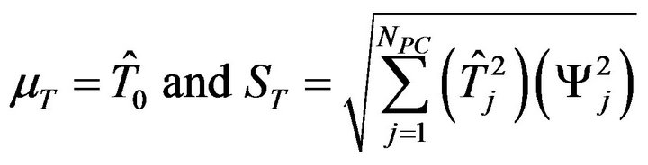
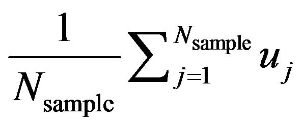
4) Generate Monte Carlo simulation results to serve as the accuracy standard in evaluating the accuracy of spectral stochastic finite element results. A Monte Carlo simulation is implemented by first sampling the thermal conductivity k according to (24). Each sample of the thermal conductivity k is then substituted into (23) to predict a sample of the temperature T. If a sufficient amount of samples of k are created, the corresponding mean value mT and standard deviation ST of temperature T will approach their exact values. These Monte Carlo simulation-based mT and ST are computed by (e.g. [1])
 (26)
(26)
where  is the total number of samples for implementing the Monte Carlo simulation, and the subscript j denotes T predicted using the j-th sample of thermal conductivity k. Meanwhile, similarly manipulating (16), the generalized polynomial chaos expansion of temperature T is
  and the corresponding spectral stochastic finite element-based predicted mT and ST are computed by (e.g. [1])
 (27)
(27)
5) Unless otherwise stated, the following parameters are adopted: 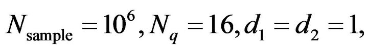
 ,
, 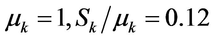 in which
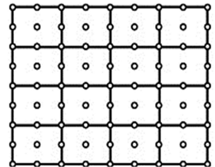

Figure 2. Finite element discretizations for analyzing the first benchmark problem (not to scale).
Nq is the total number of quadrature points in a finite element.
Furthermore, in an attempt of quantifying the errors between Monte Carlo simulation and spectral stochastic finite element results, two error estimators Dm and DS are defined below
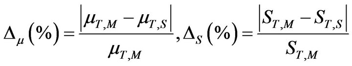 (28)
(28)
in which the subscripts M and S denote the Monte Carlo simulation and spectral stochastic finite element method; respectively.
In (28), choosing  is better checked by observing Monte Carlo simulation results with respect to different
  value. Figures 3(a) and (b) selectively checks variation of Monte Carlo simulation-based
  and
and  versus different
  values.
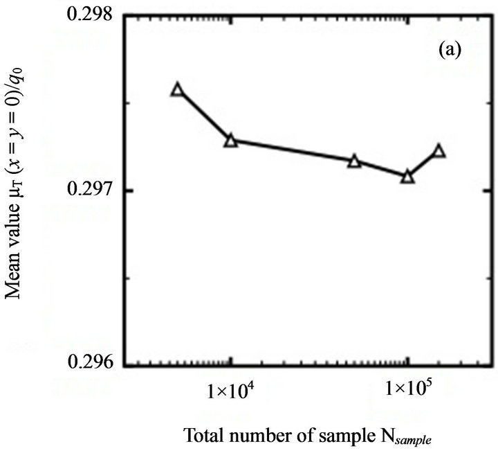
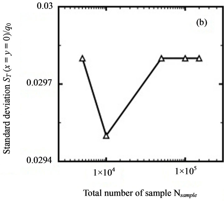
Figure 3. Variation of Monte Carlo simulation results with respect to different  values: (a) mean value; (b) standard deviation (First benchmark problem).
Although the resulting and
and  values range limitedly, Figures 3(a) and 3(b) suggest that choosing
  to implement a Monte Carlo simulation is reasonable. When more than
  samples are created, the
  and
and  values become stable.
Figures 4(a) and (b) selectively compare variation of  and
and  values with respect to Figure 2. In addition, Table 2 compares the time spent to generate spectral stochastic finite element results with adopting linear and quadratic (9-node) quadrilateral elements. Note that all essential parameters, which are not listed in Figures 4(a) and (b) and Table 2, are set according to (28). Similar practices are followed in the following.
Since we can easily expect that adopting quadratic (9-node) elements can obtain more accurate deterministic finite element results, Figure 4(a) is not surprising. Adop-
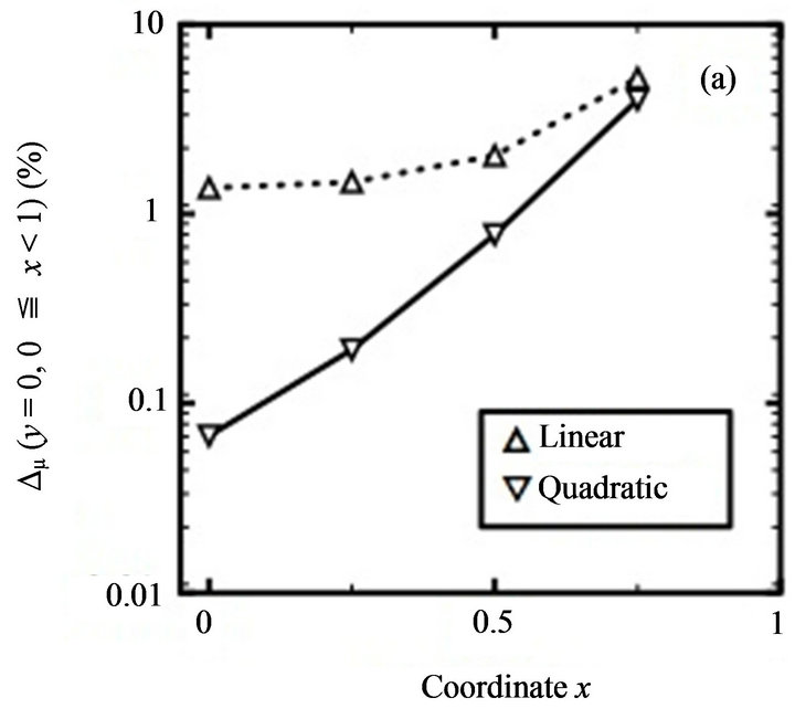
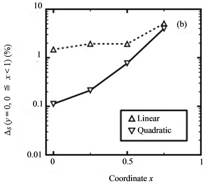
Figure 4. Comparison of accuracy of spectral stochastic finite element results with respect to linear and quadratic quadrilateral elements: (a) mean value; (b) standard deviation (First benchmark problem, m = mean value, S = standard deviation).
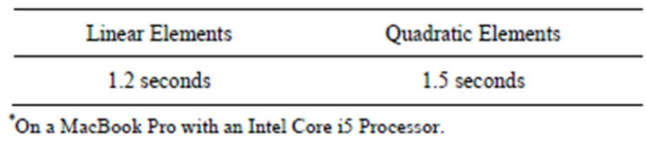
Table 2. Comparison of the time spent to generate spectral stochastic finite element results adopting linear and quadratic (9 nodes) quadrilaterals.
ting quadratic quadrilateral elements consequently predict more accurate mean values mT, since the corresponding  is smaller. Nevertheless, Figure 4(b) is surprising. Adopting quadratic (9-node) elements can also obtain more accurate predicted standard deviation ST values, since the corresponding
  values are smaller. Meanwhile, Table 2 indicates that the time spent to generate spectral stochastic finite element results is not unacceptably time-consuming.
However, we may argue that Figures 4(a) and (b) only outline the effects of spacings of any two connecting nodes on the accuracy of spectral stochastic finite elements. As the nodal distribution becomes denser, obtaining more accurate spectral stochastic finite element results may be expected. To figure out this argument, the problem domain W is re-discretized by using 64  linear quadrilateral elements and 81 equally-spaced nodes. Based on the resulting finite element discretization and Figure 2(b), Table 3 inspects variation of
  and
and  values with respect to these two cases of finite element discretization.
Inspecting Table 3 finds that adopting quadratic (9- node) elements still produces smaller  and
and values. That is, the improvement of accuracy of spectral stochastic finite element results in Figure 4(b) is not due to the denser nodal distribution in the right sub-figure of Figure 2. In fact, comparing Table 3 and Figures 4(a) and (b) finds that adopting a denser nodal distribution but still using linear elements only slightly improve the accuracy of spectral stochastic finite element results.
Furthermore, increase the  value from 0.12 to 0.32. Figures 5(a) and (b) present the corresponding
  and
and  values with respect to Figure 2. Next, change the d2 value from 1.0 to 2.0 (but revert the
  value to 0.12). Figures 6(a) and (b) present the corresponding
  and
and  values with respect to Figure 2.
The incentive of plotting Figures 5(a) and (b) comes from the published study [6] that high autocorrelation function values of stochastic coefficients (i.e. Gb values) has apparent effects on the accuracy of spectral stochastic finite element results. Further inspection of Figures 5(a) and (b) finds that adopting linear quadrilateral elements to apply the spectral stochastic finite element method
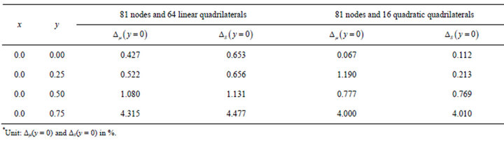
Table 3. Comparison of the time spent to generate spectral stochastic finite element results adopting linear and quadratic (9 nodes) quadrilaterals.

Figure 5. Comparison of accuracy of spectral stochastic finite element results with respect to , linear and quadratic quadrilateral elements: (a) mean value; (b) standard deviation (First benchmark problem, m = mean value, S = standard deviation).
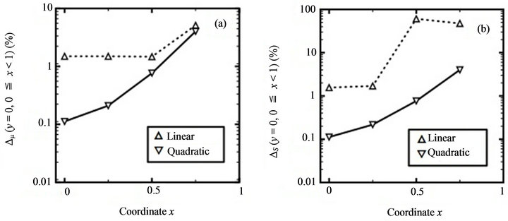
Figure 6. Comparison of accuracy of spectral stochastic finite element results with respect to d2 = 2.0, linear and quadratic quadrilateral elements: (a) mean value; (b) standard deviation (First benchmark problem, m = mean value, S = standard deviation).
may have the danger of obtaining uncontrollable  values under high Gb values. Figure 5(b) denotes an example. If linear quadrilateral elements are adopted, some
  values approach 100%. Whereas, the
  values stay below 10% when quadratic (9-node) quadrilateral elements are used. Meanwhile, Figures 6(a) and (b) indicate that the effects of different d2 values on the
  and
and  values are not noticeable. Comparing Figures 4(a) and (b) and 6(a) and (b) finds that increasing d2 values doesn’t change the
  and
and  values apparently.
3.2. Transverse Deflection of a Square Membrane
Suppose a membrane occupies a region  and
and  and its edges are fixed. Initially, the membrane is stretched so that the tension a in the membrane is uniform and that tension a is so large that it is not appreciably altered when the membrane is deflected by a distributed normal force
 .
.
To predict the transverse deflection u of the membrane, the governing equation is
 (29)
(29)
Due to symmetry, only one quadrant of the membrane is analyzed. The boundary conditions are
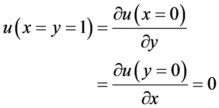 (30)
(30)
Figure 7 further illustrates the layout of problem domain W and boundary conditions. If the tension a is deterministic, the analytical solution of u is
 .
.
Meanwhile, the deterministic finite element formulation of (30) is similar to (7) except that components and
and  are; respectively
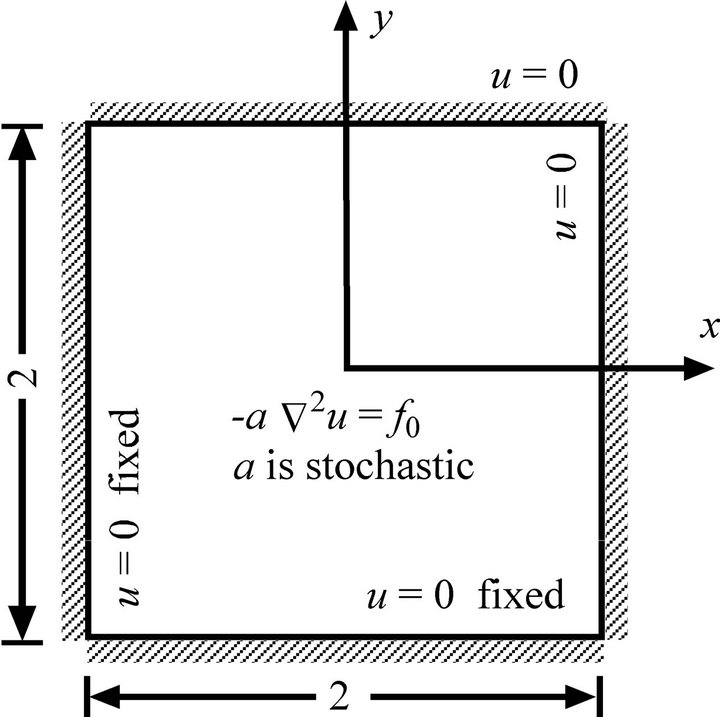
Figure 7. Transverse deflection of a square membrane (not to scale).
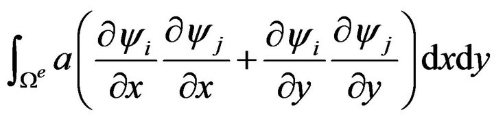 and
and .
.
Nevertheless, the succeeding study assumes the tension a varies according to the following uniform distribution:
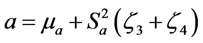 (31)
(31)
where ma and Sa are; respectively, the mean value and standard deviation of tension a,  are two random numbers.
To compare the predicted deflection u with accounting for a stochastic tension a, essential data is provided below 1) Still define W as  and
and .
.
2) Generate two cases of the finite element discretizations. As outlined by Figure 8, the left sub-figure denotes the first case which is composed of 81 nodes and 64 linear quadrilateral elements. The right sub-figure denotes the second case which is composed of. 65 nodes and 16 quadratic (8-node) quadrilateral elements.
3) Consulting with Table 1, represent a by the Legendre polynomial chaos.
4) Generate Monte Carlo simulation results by first sampling the tension a according to (31). Each sample of the tension a is then substituted into the aforementioned analytical solution of (29) to predict a sample of the deflection u. Similarly manipulating (26), the mean value mu and standard deviation Su of deflection u are equal to
 and
and ;
;
respectively. Meanwhile, the spectral stochastic finite element-based predicted mu and Su are equal to  and
and
 ; respectively in which
  (
( to
to
 ) is obtained from the generalized polynomial chaos expansion of u.
5) Unless otherwise stated, the following parameters are adopted:
 ,
, .
.
Similarly manipulating Section 3.1, variation of the Monte Carlo simulation results versus different  values and the accuracy of spectral stochastic finite element
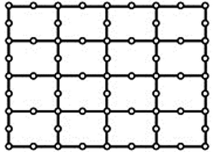
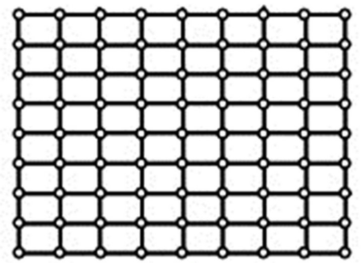
Figure 8. Finite element discretizations for analyzing the second benchmark problem (not to scale).
results are evaluated as follows: Figures 9(a) and (b) evaluate variation of Monte Carlo simulation-based predicted  and
and  with respect to different
  values. Figures 10(a) and (b) present variation of
and

values with respect to Figure 8. Figures 11(a) and (b) compare variation of  and
and  values with respect to Figure 8 and
 .
.
Figures 9(a) and (b) report that choosing  is still reasonable. As the
  value is larger than 106, the Monte Carlo simulation-based predicted
 and
and  remain approximately fixed. Meanwhile, we still find from Figures 10(a) and (b) that adopting quadratic (8-node) elements is conducive to improving the accuracy of spectral stochastic finite elmentbased predicted
 , since the corresponding
  value is smaller. Note that the total number of nodes in the left sub-figure of Figure 8 is more than the total number of nodes in the right sub-figure of the same figure. Since similar results are found in Table 3 and Figures 4(a) and (b), adopting more nodes but still using the same element type consequently improve the accuracy of corresponding spectral stochastic finite element results slightly.
On the other hand, comparing Figures 10(a) and (b) with Figures 11(a) and (b) finds that
 and
and 
values further increases versus the increase of  values and the left sub-figure of Figure 8. Howeverthe
 value in Figure 11(b) doesn’t approach 100 %. This experience implies that different probability distributions of stochastic coefficients can produce different patterns of spectral stochastic finite element-based predicted mean values and standard deviations. Hence, the current study suggests doing some pilot tests to observe the performance of spectral stochastic finite element method versus a specific probability distribution of stochastic coefficients before practically applying this probability distribution.
4. Closure
As introduced in Section 1, the most popular numerical tool for solving stochastic partial differential equations may be the spectral stochastic finite element method. Numerous resources are available for generating spectral stochastic finite element results. As compared to the Monte Carlo simulation, applying the spectral stochastic finite element method doesn’t require sampling the existing random fields sufficiently; thus, creating spectral stochastic finite element results is usually time-saving.
Probably since deterministic analytical solutions are usually unavailable for producing Monte Carlo simulation results, the accuracy of spectral stochastic is not often discussed and linear elements were usually adopted in applying this stochastic numerical method. However, the succeeding study demonstrates that adopting highorder (e.g. quadratic) elements can improve the performance of spectral stochastic finite element method. The previous section has shown that adopting linear elements has the danger of obtaining uncontrollable errors between Monte Carlo simulation and spectral stochastic finite element results. Whereas, adopting quadratic (9-node or 8-node) elements to apply the spectral stochastic finite element method stably produces more accurate predicted
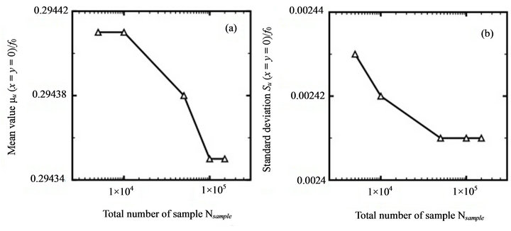
Figure 9. Variation of Monte Carlo simulation results with respect to different Nsample values: (a) mean value; (b) standard deviation (Second benchmark problem).
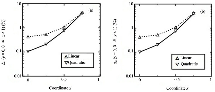
Figure 10. Comparison of accuracy of spectral stochastic finite element results with respect to linear and quadratic quadrilateral elements: (a) mean value; (b) standard deviation (Second benchmark problem, m = mean value, S = standard deviation).
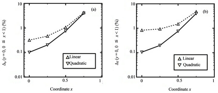
Figure 11. Comparison of accuracy of spectral stochastic finite element results with respect to , linear and quadratic quadrilateral elements: (a) mean value; (b) standard deviation (Second benchmark problem, m = mean value, S = standard deviation).
mean values and standard deviations under high autocorrelation function values of existing stochastic coefficients ranges. In addition, the time spent to apply the spectral stochastic finite element method with using quadratic quadrilateral elements is not unacceptably time-consuming.
In conclusion, replacing linear elements with highorder elements to apply the spectral stochastic finite element method can be as a low-cost method to improve the performance of this stochastic numerical method.
REFERENCES
- R. G. Ghanem and P. D. Spanos, “Stochastic Finite Elements: A Spectral Approach,” Springer-Verlag, New York, 2012.
- D. Xiu and G. E. Karniadakis, “Modeling Uncertainty in Flow Simulations via Generalized Polynomial Chaos,” Journal of Computational Physics, Vol. 187, No. 1, 2003, pp. 137-167. doi:10.1016/S0021-9991(03)00092-5
- M. Loève, “Probability Theory II (Graduate Text in Mathematics),” Springer-Verlag, Berlin, 1978.
- S. Q. Wu and S. S. Law, “Evaluating the Response Statistics of an Uncertain Bridge-vehicle System,” Mechanical Systems and Signal Processing, Vol. 27, 2012, pp. 576- 589. doi:10.1016/j.ymssp.2011.07.019
- V. Papadopoulos and O. Kokkinos, “Variability Response Functions for Stochastic Systems,” Probabilistic Engineering Mechanics, Vol. 28, 2012, pp. 176-184. doi:10.1016/j.probengmech.2011.08.002
- G. Y. Sheu, “Prediction of Probabilistic Settlements via Spectral Stochastic Meshless Local Petrov-Galerkin Method,” Computers and Geotechnics, Vol. 38, No. 4, 2011, pp. 407-415. doi:10.1016/j.compgeo.2011.02.001
- M. F. Ngah and A. Young “Application of the Spectral Stochastic Finite Element Method for Performance Prediction of Composite Structures,” Composite Structures, Vol. 78, No. 3, 2007, pp. 447-456. doi:10.1016/j.compstruct.2005.11.009
- J. N. Reddy, “An Introduction to the Finite Element Method,” 2nd Edition, McGraw-Hill Company, New York, 1993.