Applied Mathematics
Vol.4 No.8(2013), Article ID:35095,6 pages DOI:10.4236/am.2013.48150
On Some Procedures Based on Fisher’s Inverse Chi-Square Statistic
Department of Biostatistics, Bioinformatics, and Biomathematics, Georgetown University, Washington DC, USA
Email: khm33@georgetown.edu
Copyright © 2013 Kepher H. Makambi. This is an open access article distributed under the Creative Commons Attribution License, which permits unrestricted use, distribution, and reproduction in any medium, provided the original work is properly cited.
Received February 1, 2013; revised March 1, 2013; accepted March 9, 2013
Keywords:  Values; Weighting; Linear Combination; Correlation Coefficient; Estimated Degrees of Freedom
ABSTRACT
We present approximations to the distribution of the weighted combination of independent and dependent  values,
 ![]() In case that independence of
In case that independence of ’s is not assumed, it is argued that the quantity
  is implicitly dominated by positive definite quadratic forms that induce a chi-square distribution. This gives way to the approximation of the associated degrees of freedom using Satterthwaite (1946) or Patnaik (1949) method. An approximation by Brown (1975) is used to estimate the covariance between the log transformed
  -values. The performance of the approximations is compared using simulations. For both the independent and dependent cases, the approximations are shown to yield probability values close to the nominal level, even for arbitrary weights,
 ’s.
’s.
1. Introduction
Let  be
be ![]() tail probabilities or probability values from continuous distributions. Associate null hypotheses
tail probabilities or probability values from continuous distributions. Associate null hypotheses  to these
 ![]() probability values. Using the probability integral transform, we know that
probability values. Using the probability integral transform, we know that  when
when  is true. For
That is,  which is the cumulative distribution function of a chi-square variable with 2 degrees of freedom. That is,
  and the decision rule is to reject
  if
if  Define a combined statistic by
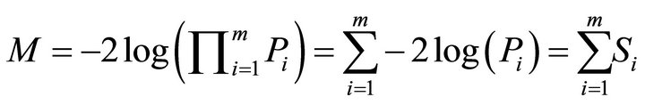
For independent ’s, the variable
  The overall test procedure is to reject
  if
if  This is Fisher’s Inverse Chi-square method. We notice that for the statistic
  all the
 ’s are weighted equally, which may not be acceptable in some situations and therefore unequal weighting may be necessary. A number of authors have attempted to derive the distribution of a weighted form of
  For instancelet
  where
where  has a non-central
 distribution with non-centrality parameter
  Solomon and Stephens [1] approximated the distribution of
  by a random variable of the form
matching the first three moments. The disadvantage with this approximation is that there is no closed-form formula for computing the parameters. Buckley and Eagleson [2] approximation of the distribution of  involves approximating
  using a variable that takes the form
  and matching the first three cumulants of
 ![]() and
and  Zhang [3] showed that by equating the first three cumulants of
  and
and  the distribution of
  can be approximated by
  Zhang [3] also proposed a chi-square approximation to the distribution of
  Others authors have approximated the null distribution of
  by intensive bootstrap [4-8].
In this article, we concentrate on linear combinations of  (a function of
 ’s) that have a central chi-square distribution, and involve dependent and independent
 ’s and arbitrary weights,
 ’s. For dependent
 ’s, we use simulations to investigate the performance of the approach by Makambi [9] when it is assumed that there is homogeneity in correlation coefficients between any pair of the
 ’s.
’s.
2. Distribution of Independent and Dependent Weighted ’s
’s
Let’s focus on the mixture
where  has a central
  -distribution with 2 degrees of freedom and
  are arbitrary weights. For independent
 ’s, Good [10] provided the following approximation:
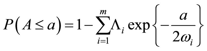
where 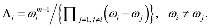 This approximation is usually regarded as the exact distribution of
  The approximation has been criticized because the calculations become ill-conditioned when any two weights,
  and
and  are equal. To avoid this problem, Bhoj [11] proposed the approximation
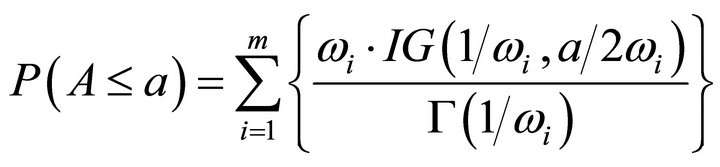
where  denotes the incomplete gamma function. This approximation is also for independent probability values.
For an alternative and more general approximation to the distribution of  where independence of
 ’s is not assumed, it may be argued that
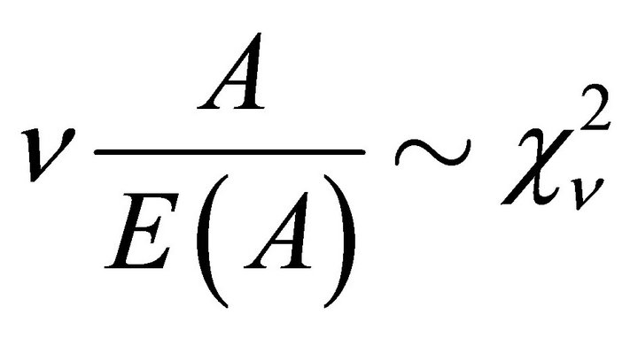
  is a quantity that is implicitly dominated by positive definite quadratic forms that induce a chi-square distribution. Thus by Satterthwaite [12] or Patnaik [13], we have
It follows that
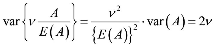
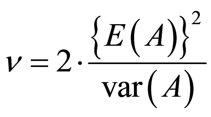
Therefore, the degrees of freedom can be obtained by solving the above equation for  namely,
Now,
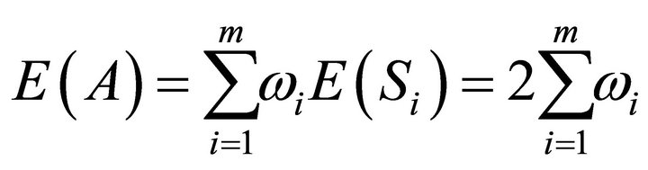
and
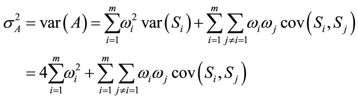
where  denotes the covariance between
  and
and  for
for  An estimate of the degrees of freedom,
  is given by
  (see [9,14]).
We can now synthesize the ![]() probability values
probability values  based on the decision rule
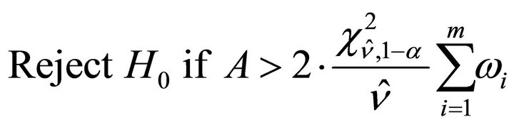
For normalized weights, that is,  the decision rule is:
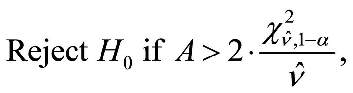
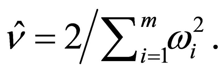
with an estimate of the degrees of freedom ![]() given by
given by  Notice that for independent
  and
and  and normalized weights, Makambi [9] and Hou [14] utilize
 For
For  and 4, Hou [14] presented simulation results indicating that the approximation given above attains probability values close to the nominal level, similar to the Good [10] and Bhoj [11] approximations.
For  independent
  -values, we use Table 1 in Hou [14] to obtain Table 1, just for purposes of comparing the performance of the approaches. We notice that using
  (column 5, Table 1) yields results that are close to both the exact method by Good [10] and the method by Bhoj [11].
To illustrate the application of the methods for independent probability values, we use data from Canner [15] on four selected multicenter trials involving aspirin and post-myocardial infarction patients carried out in Europe and the United States in the period 1970-1979. Two of these trials, referred to as UK-1 and UK-2 were carried out in the United Kingdom; the Coronary Drug Project Aspirin Study (CDPA); and the Persantine-Aspirin Reinfarction Study (PARIS) (Table 2).
The  values provided in column 4 of Table 2 are for the log odds ratio as the outcome measure of interest. Using the
  values in Table 2 and the weights from Table 1 of [14], we obtain the values in Tables 3. We have also included results for normalized inverse variance weights determined from the data. The three approximations yield values that are close to each other, and are in good agreement with the exact method by Good [10].
If  and
and  are non-independent, the expression for
  contains a covariance term between
  and
and  that has to be estimated. Let
  be the correlation between
  and
and  i.e.,
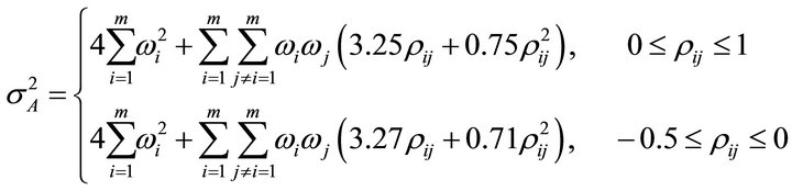
i.e.,  An approximation of the variance of
  is given by [16]
3. A Procedure for Constant Correlation Coefficient
We require estimates of  to implement the procedures above for dependent
 ’s. Let’s consider the case of homogeneous nonnegative correlation coefficients, that is,
  for
for  Let
Let  and define the quadratic form [9]
We can write 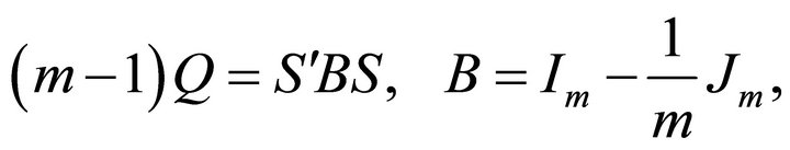
where  is identity matrix of order
 ![]() and
and  is a square matrix of order
 ![]() with every element equal to unity. It can be shown that
with every element equal to unity. It can be shown that 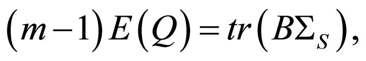
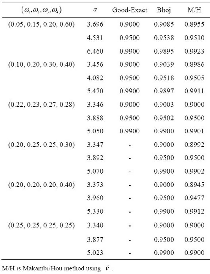
Table 1.  for independent
 ’s.
’s.
where 
 and
and
 is the trace of the matrix
  For homogeneous
 and using results from Brown [16] we have
 ![]() We can show that
We can show that  Solving the preceding equation for
  yields the approximate admissible solution
 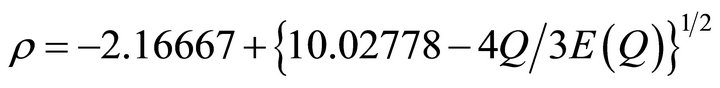 with an estimate for
  given by
 (1)
(1)
We investigate how well this approximation works compared with the other approximations by simulating data from a ![]() variate normal distribution with covariance matrix
variate normal distribution with covariance matrix  with
with  and
and  Just as in Hou [14], we simulated
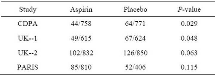
Table 2. Data on total mortality in six aspirin trials (Number of Deaths/Number of patients).
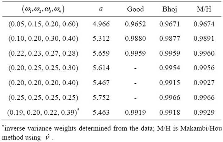
Table 3.  for independent
 ’s using Canner (1987) data for
 .
.
10,000 multivariate normal samples and computed the corresponding values of  For
For  and 4, we present values for
  at selected nominal levels and weights (Tables 4-6).
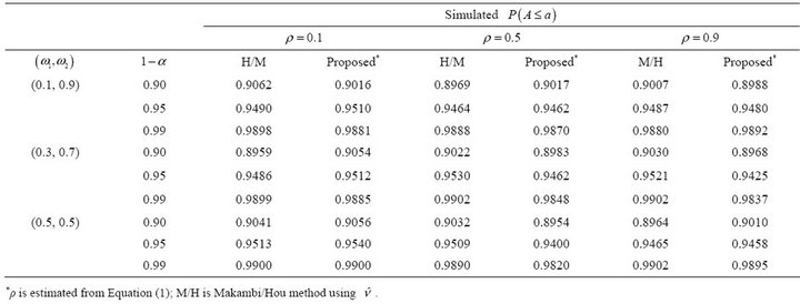
Table 4. Simulated estimates of  at selected nominal levels for non-independent
 ’s from bivariate normal distribution with
 ![]() and covariance matrix
and covariance matrix  with
with  and
and .
.
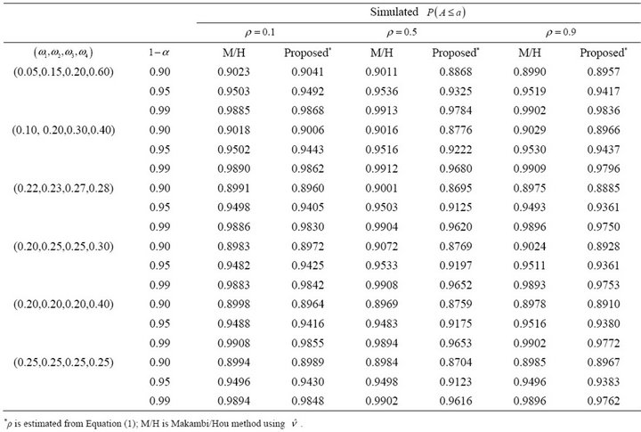
Table 5. Simulated estimates of  at selected nominal levels for non-independent
 ’s from multivariate normal distribution with
 ![]() and covariance matrix
and covariance matrix  with
with  and
and 
 .
.
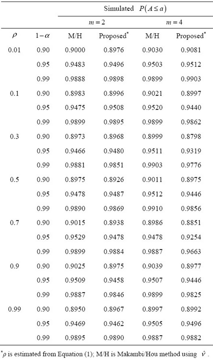
Table 6. Simulated estimates of 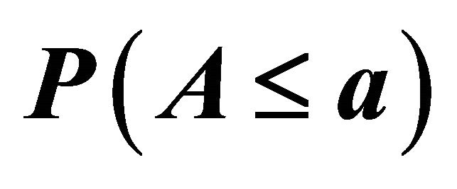 (with weights,
  simulated from
 ) at selected nominal levels for non-independent
 ’s from bivariate normal distribution with
 ![]() and covariance matrix
and covariance matrix  with
with  and
and .
.
For  (Table 4) the proposed method attains probability levels that are close to the nominal level, similar to the Makambi/Hou method.
For  (Table 5) the proposed estimate of the constant correlation coefficient
  leads to attained probability level that are close to the nominal level,
  for
for  and 0.9. However, for values of
  close to 0.5, the estimate leads to underestimation of the probability level.
Now, instead of using pre-defined weights, we simulated weights from a beta distribution with parameters  and
and  That is, for
 such that
  Results are given in Table 6 for selected nominal levels.
4. Conclusion
In this article, we have presented chi-square approximations to the distribution of Fisher’s inverse chi-square statistic for independent and dependent  values. It has also been shown that, for dependent
  values, the proposed estimate of the constant correlation coefficient
  performs well by attaining probability levels close to the nominal level for correlation coefficients close to 0.1 and 0.9. We expect the proposed estimate to underestimate probability levels for relatively large numbers of studies, especially when
  is close to 0.5. However, for values close to 0.1 and 0.9, the proposed estimate works quite well and can be recommended.
REFERENCES
- H. Solomon and M. A. Stephens, “Distribution of a Weighted Sum of Chi-Squared Variables,” Journal of the American Statistical Association, Vol. 72, No. 360a, 1977, pp. 881-885.
- M. J. Buckley and G. G. Eagleson, “An Approximation to the Distribution of Quadratic Forms in Normal Random Variables,” Australian Journal of Statistics, Vol. 30A, No. 1, 1988, pp. 150-159. doi:10.1111/j.1467-842X.1988.tb00471.x
- J.-T. Zhang, “Approximate and Asymptotic Distributions of Chi-Squared-Type Mixtures with Applications,” Journal of the American Statistical Association, Vol. 100, No. 469, 2005, pp. 273-285. doi:10.1198/016214504000000575
- R. L. Eubank and C. H. Spiegelman, “Testing the Goodness of Fit of a Linear Model via Non-Parametric Regression techniques,” Journal of the American Statistical Association, Vol. 85, No. 410, 1990, pp. 387-392. doi:10.1080/01621459.1990.10476211
- A. Azzalini and A. W. Bowman, “On the Use of NonParametric Regression for Checking Linear Relationships,” Journal of the Royal Statistical Society Series B, Vol. 55, No. 2, 1993, pp. 549-557.
- J. C. Chen, “Testing the Goodness of Fit of Polynomial Models via Spline Smoothing Techniques,” Statistics and Probability Letters, Vol. 19, No. 1, 1994, pp. 65-76. doi:10.1016/0167-7152(94)90070-1
- W. Gonzalez-Manteiga and R. Cao, “Testing the Hypothesis of a General Linear Model Using Non-Parametric Regression Estimation,” Test, Vol. 2, No. 1-2, 1993, pp. 161-188. doi:10.1007/BF02562674
- J. Fan, C. Zhang, J. Zhang, “Generalized Likelihood Ratio Statistics and Wilks Phenomenon,” The Annals of Statistics, Vol. 29, No. 1, 2001, pp. 153-193. doi:10.1214/aos/996986505
- K. H. Makambi, “Weighted Inverse Chi-Square Method for Correlated Significance Tests,” Journal of Applied Statistics, Vol. 30, No. 2, 2003, pp. 225-234. doi:10.1080/0266476022000023767
- I. J. Good, “On the Weighted Combination of Significance Tests,” Journal of the Royal Statistical Society Series B, Vol. 17, No. 1, 1995, pp. 264-265.
- D. S. Bhoj, “On the Distribution of the Weighted Combination of Independent Probabilities,” Statistics & Probability Letters, Vol. 15, No. 1, 1992, pp. 37-40. doi:10.1016/0167-7152(92)90282-A
- F. E. Satterthwaite, “An Approximate Distribution of the Estimates of Variance Components,” Biometrics Bulletin, Vol. 2, No. 6, 1946, pp. 110-114. doi:10.2307/3002019
- P. B. Patnaik, “The Non-Central
 -and
-and  -Distributions and Their Applications,” Biometrika, Vol. 36, No. 1-2, 1049, pp. 202-232.
 - C. D. Hou, “A Simple Approximation for the Distribution of the Weighted Combination of Nonindependent or Independent Probabilities,” Statistics and Probability Letters, Vol. 73, No. 2, 2005, pp. 179-187. doi:10.1016/j.spl.2004.11.028
- P. L. Canner, “An Overview of Six Clinical Trials of Aspirin in the Coronary Heart Disease,” Statistics in Medicine, Vol. 6, No. 3, 1987, pp. 255-263.
- M. B. Brown, “A Method for combining Non-Independent, One-Sided Tests of Significance,” Biometrics, Vol. 31, No. 4, 1975, pp. 987-992. doi:10.2307/2529826