Applied Mathematics
Vol.4 No.2(2013), Article ID:28188,5 pages DOI:10.4236/am.2013.42043
What Is the Difference between Gamma and Gaussian Distributions?
School of Electrical Engineering and Computer Science, University of Newcastle, Newcastle, Australia
Email: xiaoli.hu@newcsatle.edu.au, xlhu@amss.ac.cn
Received November 19, 2012; revised December 25, 2012; accepted January 3, 2013
Keywords: Gamma Distribution; Gaussian Distribution; Berry-Esseen Inequality; Characteristic Function
ABSTRACT
An inequality describing the difference between Gamma and Gaussian distributions is derived. The asymptotic bound is much better than by existing uniform bound from Berry-Esseen inequality.
1. Introduction
1.1. Problem
We first introduce some notations. Denote Gamma distribution function as
 (1)
(1)
for  and
and , where
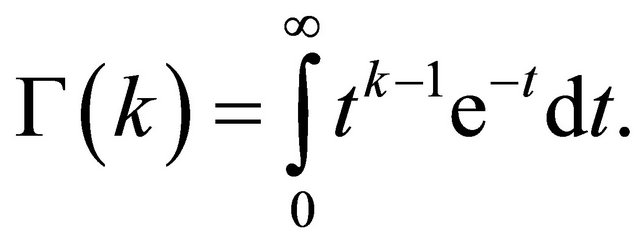
  is the Gamma function, i.e.,
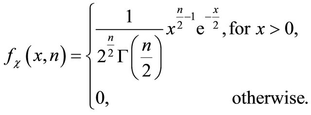
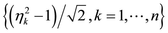
Assume  for
for . The density of chisquare distributed random variable
  with
with ![]() degrees of freedom is
degrees of freedom is
It is well-known that the random variable ![]() can be interpreted by
can be interpreted by 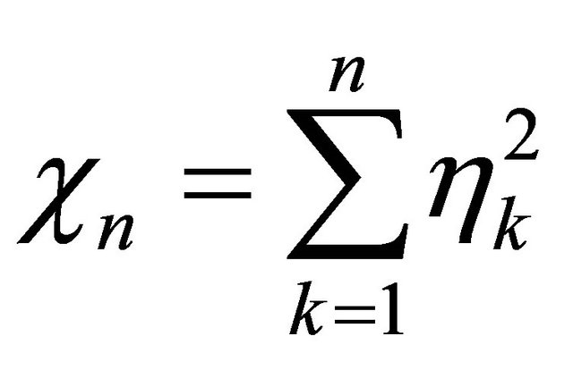 with
with ![]() independent and identically distributed (i.i.d.) random variables
independent and identically distributed (i.i.d.) random variables 
 where
where  denotes the standard Gaussian distribution. The mean and variance of
  is respectively
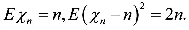
Then, by simple change of variable we find
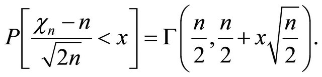 (2)
(2)
On the other side, by the Berry-Esseen inequality to
 , it is easy to find a bound
 such that
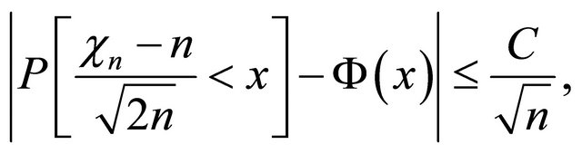 (3)
(3)
where  is the standard Gaussian distribution function, i.e.,
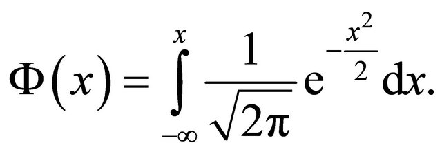 (4)
(4)
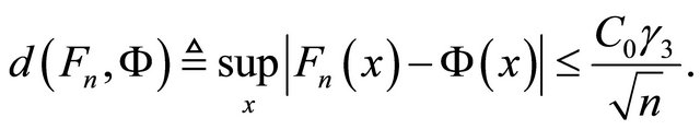
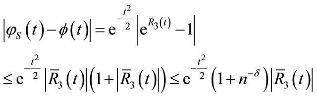
Then, by Equations (2) and (3) it follows
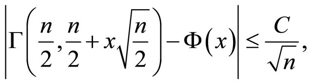 (5)
(5)
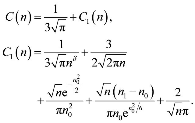
which describes the distance between Gamma and Gaussian distributions. The purpose of this paper is to derive asymptotic sharper bound  in Equation (5), which much improves the constant
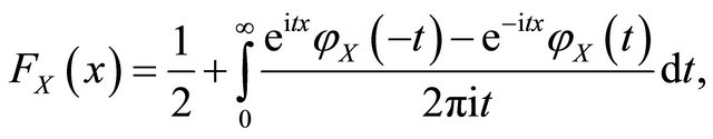
  by directly using Berry-Esseen inequality. The main framework of analysis is based on Gil-Pelaez formula (essentially equivalent to Levy inversion formula), which represents distribution function of a random variable by its characteristic function.
The main result of this paper is as following.
Theorem 1.1 A relation of the Gamma distribution (1) and Gaussian distribution (4) is given by
 (6)
(6)
where
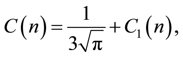
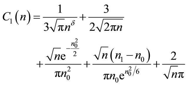
with 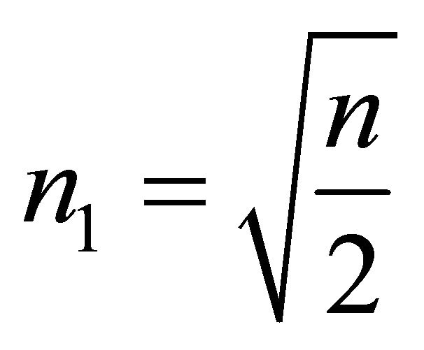 and
and  for any
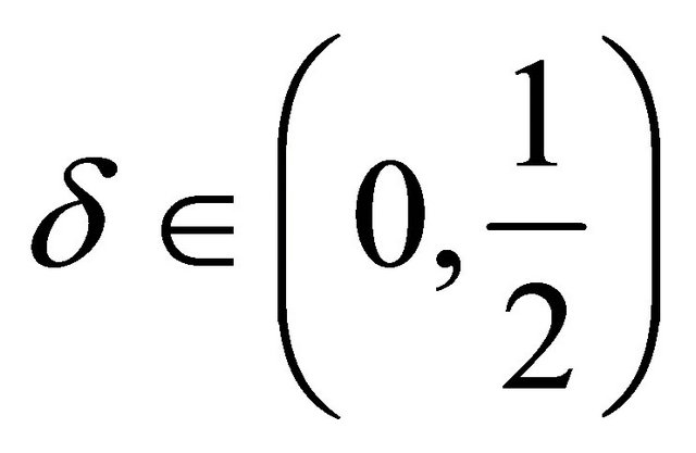 .
.
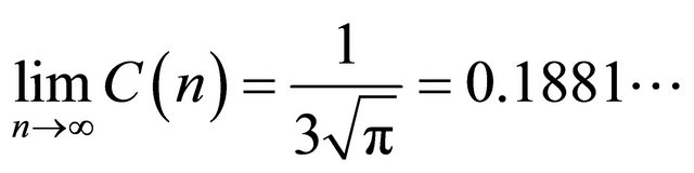
Clearly,  as
as![]() . Thus, the asymptotical bound is
. Thus, the asymptotical bound is
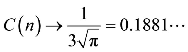
as![]() . To check the tightness of the limit value of
. To check the tightness of the limit value of , we plot in Figure 1 the multiplication
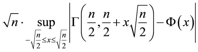
for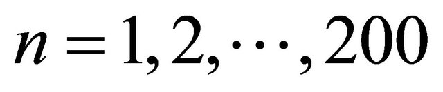 , where the straight line is the limit value
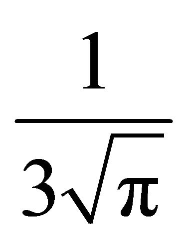 . From this experiment it seems that
is the best constant. The tendency of the theoretical formula 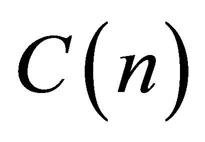 is plotted for
 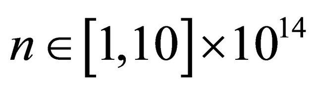 in Figure 2, which also shows the tendency to the limit value
 . The slow trend is due to that some upper bounds formulated over interval
 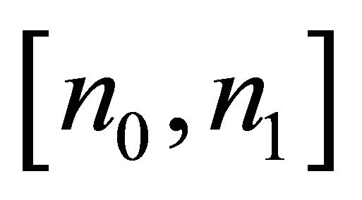 have been weakly estimated, e.g., the third and fourth terms of
 .
.
1.2. Comparison to the Bound Derived by Berry-Esseen Inequality
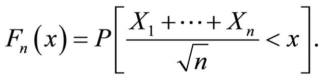
Let  be a sequence of independent identically distributed random variables with EX1 = 0
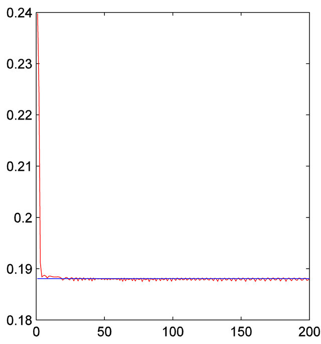
Figure 1. Experiment.
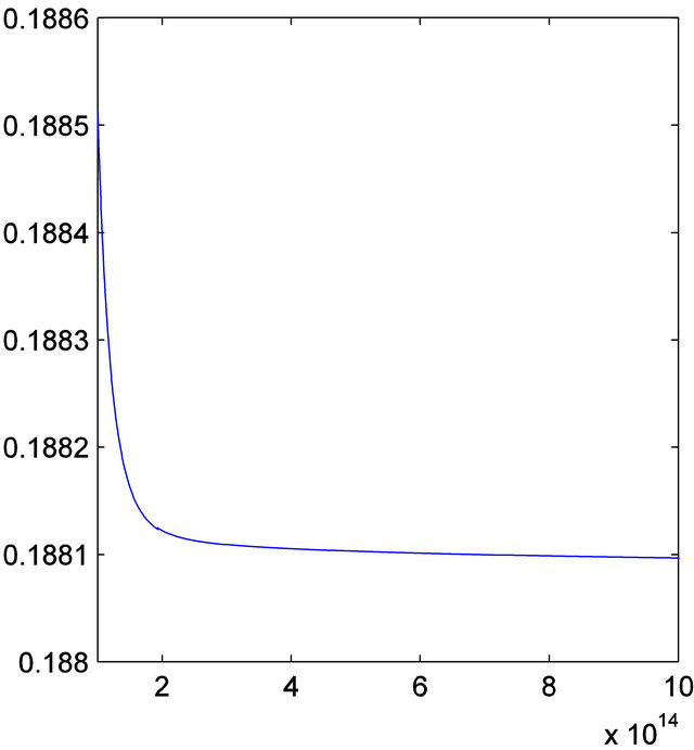
Figure 2. Trend of .
.
and finite third absolute moment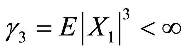 . Denote
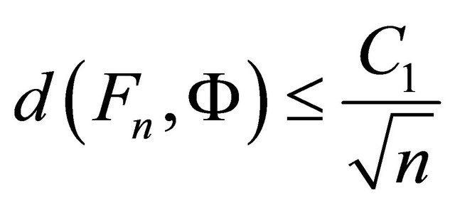
By classic Berry-Esseen inequality, there exists a finite positive number  such that
 (7)
(7)
The best upper bound 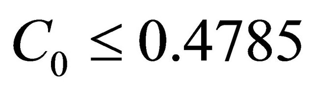 is found in [1] in 2009. The bound is improved in [2] at some angle in a slight different form as
 (8)
(8)
with

The inequality (8) will be sharper than Equation (7) for .
.
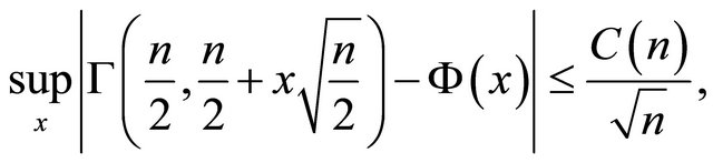
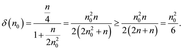
Now let us derive the constant  in (5) by applying Berry-Esseen inequality to
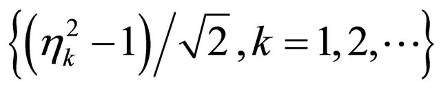 . It is difficult to calculate the exact value of third absolute moment of the random variable
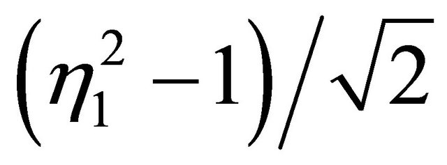 . Thus, it is approximated as
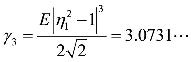
by using Matlab to integrate over interval  divided equivalently 100,000 subinterval for its half value.
By Equation (7) with 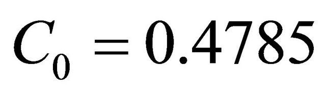 we have
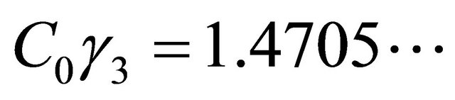
and by Equation (8) we have
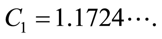
Hence, the best constant  in Equation (5) by applying Berry-Esseen inequality is
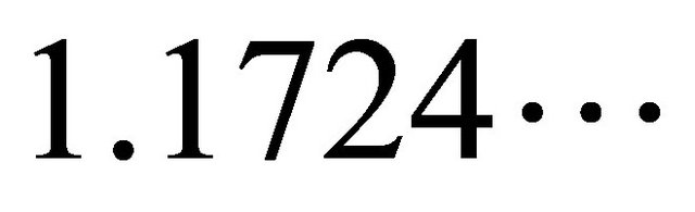 . Obviously, the limit bound
found in this paper for chi-square distribution is much better.
The technical reason is that the Berry-Esseen inequality deals with general i.i.d. random sequences without exact information of the distribution.
2. Proof of Main Result
Before to prove the main result, we first list a few lemmas and introduce some facts of characteristic function theory.
2.1. Some Lemmas
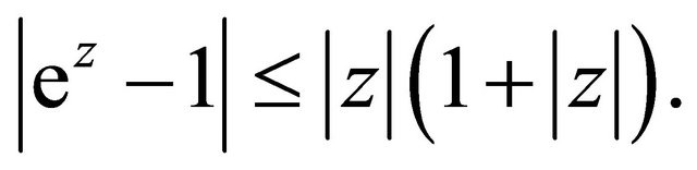
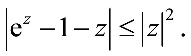
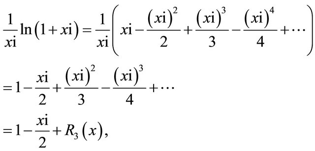
Lemma 2.1 For a complex number  satisfying
 ,
, 
Proof First show that
By Taylor’s expansion and noting , we have
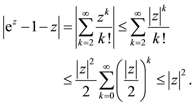
Together with
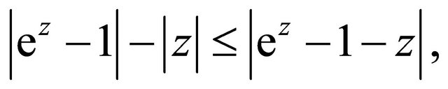
the assertion follows.
Lemma 2.2 For a real number ![]() satisfying
satisfying ,
,
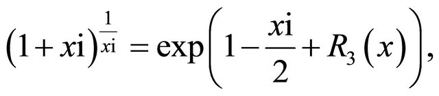
where  is the imaginary unit and
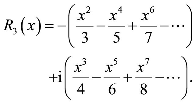
Clearly,
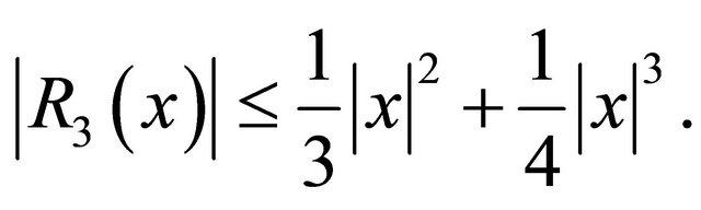
Proof. By Taylor expansion for complex function, for  we have
where 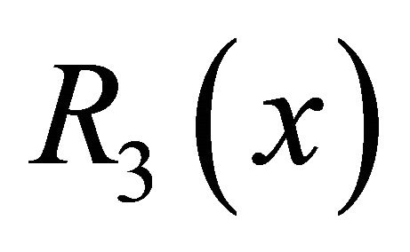 is shown above. By further noting the two alternating real series above, it follows the upper bound.
We cite below a well-known inequality [3] as a lemma.
Lemma 2.3 The tail probability of the standard normal distribution satisfies
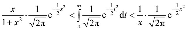
for .
.
2.2. Characteristic Function
Let us recall, see e.g., [4], the definition and some basic facts of characteristic function (CF), which provides another way to describe the distribution function of a random variable. The characteristic function of a random variable  is defined by
where  is the imaginary unit, and
  is the argument of the function. Clearly, the CF for random variable
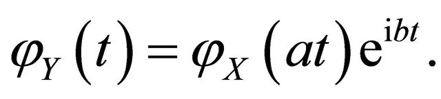
  with real numbers
 ![]() and
and  is
is
Another basic quality is
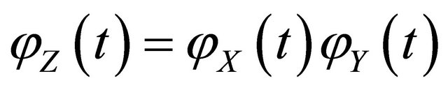
for 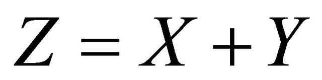 with
with  and
and ![]() independent to each other.
independent to each other.
It is well-known that the CF of standard Gaussian  is
is
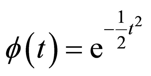 (9)
(9)
and the CF of chi-square distributed variable  is
is
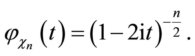
Thus, the CF for 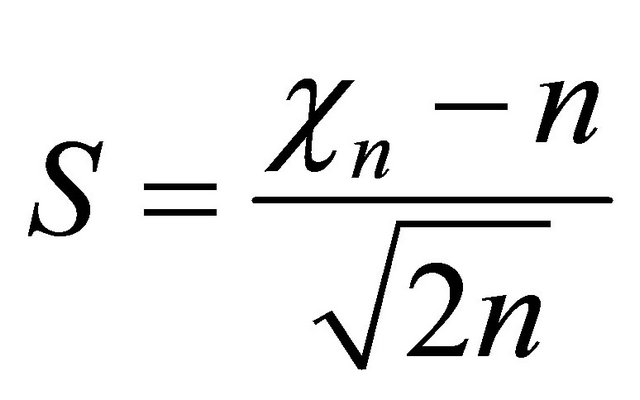 is
is
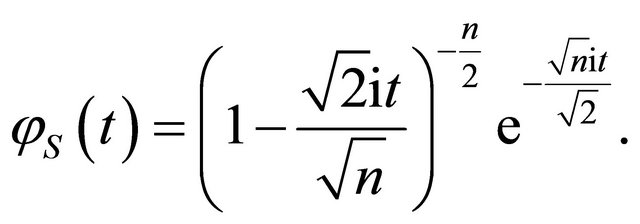 (10)
(10)
The CF is actually an inverse Fourier transformation of density function. Therefore, distribution function can be expressed by CF directly, e.g., Levy inversion formula. We use another slightly simpler formula. For a univariate random variable , if
, if ![]() is a continuity point of its distribution
is a continuity point of its distribution , then
 (11)
(11)
which is called Gil-Pelaez formula, see, e.g., page 168 of [4].
2.3. Proof of Main Result
We are now in a position to prove the main result.
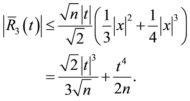
Proof of Theorem 1.1 First analyze CF of 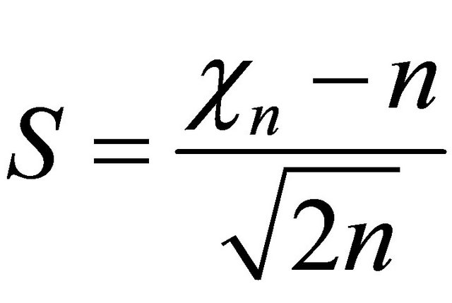 given by Equation (10). Denote
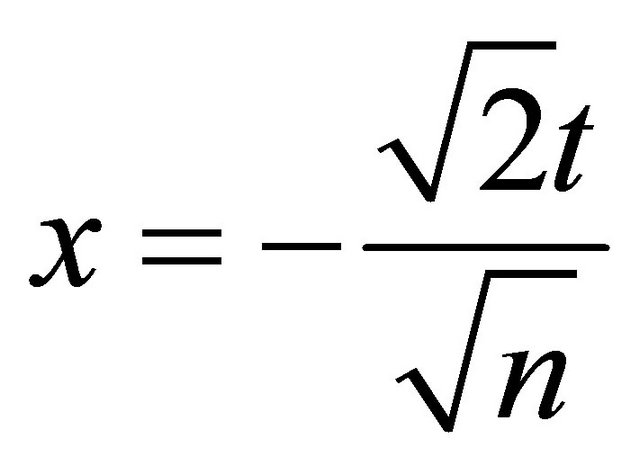 . For
. For , i.e.,
 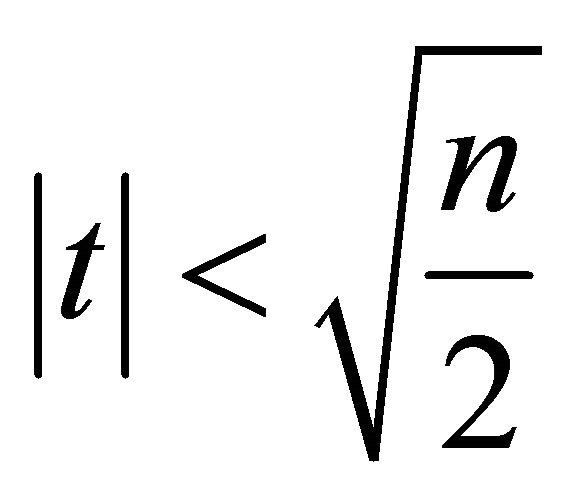 , by Lemma 2.2,
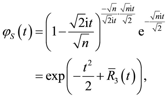 (12)
(12)
where
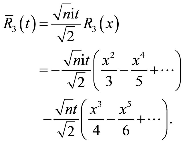
Clearly,
To make sure 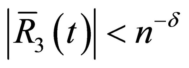 for some
 denote
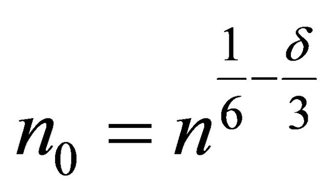 . Then, it is easy to see that
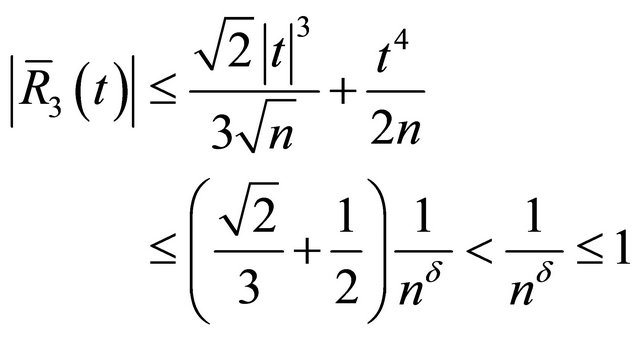 (13)
(13)
for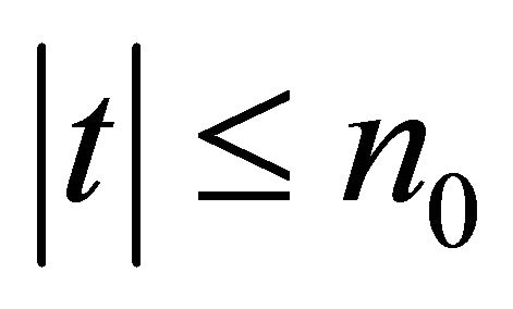 . Hence, by Equations (12) and (13) and Lemma 2.1,
 (14)
(14)
for .
.
Now let us consider the difference between  and
and , i.e., the CF (9) of Gaussian distribution, over the interval
 . By Equation (14)
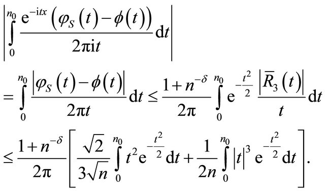
Note that
it follows
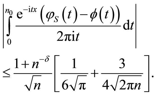 (15)
(15)
Similarly,
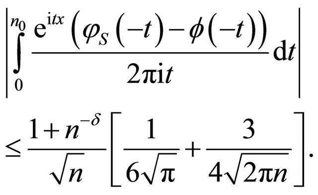 (16)
(16)
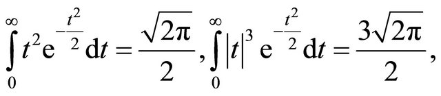
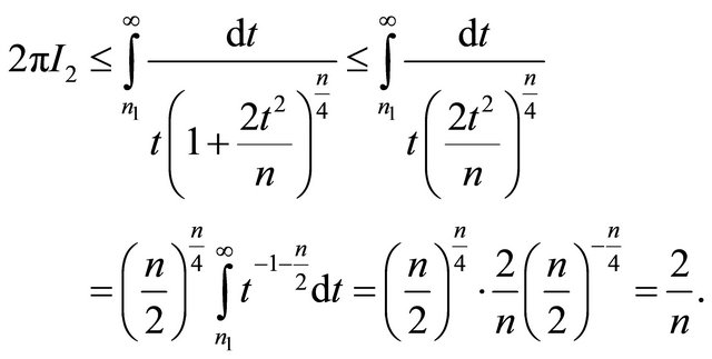
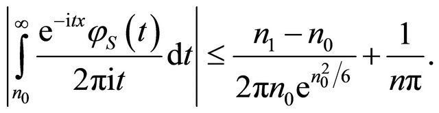
Below let us analyze the residual integrals over the interval . By Lemma 2.3,
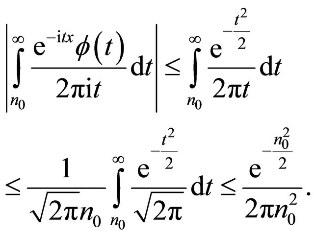 (17)
(17)
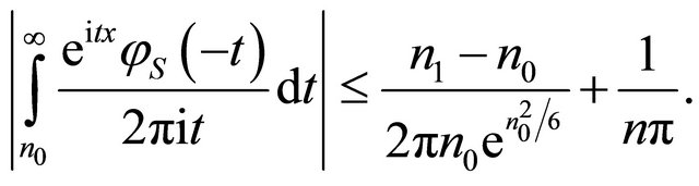
Similarly,
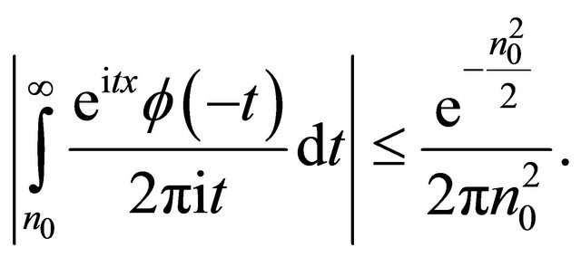 (18)
(18)
It is somewhat difficult to analyze the residual integral over  for
for . We divide it into two subintervals as following:
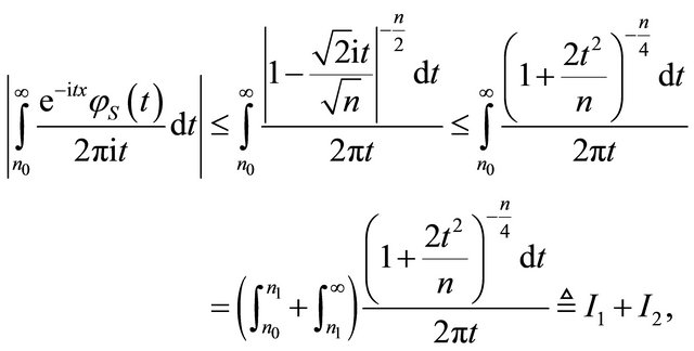
where .
.
Observe that  decreases on interval
  and
and  for
for , we have
where
The fact  is used in above formula. Thus,
 (19)
(19)
For the other interval , we proceed as
 (20)
(20)
By Equations (19) and (20)
 (21)
(21)
Similarly,
 (22)
(22)
By Equation (15), Equation (17), Equation (21) and Equation (16), Equation (18), Equation (22)
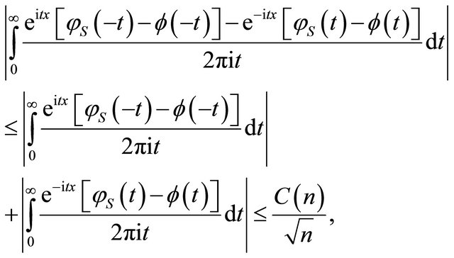
where
In view of Formula (11) , the formula to be proved follows directly.
REFERENCES
- I. S. Tyurin, “On the Accuracy of the Gaussian Approximation,” Doklady Mathematics, Vol. 80, No. 3, 2009, pp. 840-843. doi:10.1134/S1064562409060155
- V. Koroleva and I. Shevtsova, “An Improvement of the Berry-Essen in Equality with Application to Possion and Mixed Poison Random Sums,” Scandinavian Actuarial Journal, Vol. 2012, No. 2, 2012, pp. 81-105. doi:10.1080/03461238.2010.485370
- R. D. Gordon, “Values of Mills’ Ratio of Area to Bounding Ordinate and of the Normal Probability Integral for Large Values of the Argument,” The Annals of Mathematical Statistics, Vol. 12, No. 3, 1941, pp. 364-366. doi:10.1214/aoms/1177731721
- K. L. Chung, “A Course in Probability Theory,” 3rd Edition, Probability and Mathematical Statistics, Academic, New York, 2001.