ABSTRACT

We explore the stability of image reconstruction algorithms under deterministic compressed sensing. Recently, we have proposed [1-3] deterministic compressed sensing algorithms for 2D images. These algorithms are suitable when Daubechies wavelets are used as the sparsifying basis. In the initial work, we have shown that the algorithms perform well for images with sparse wavelets coefficients. In this work, we address the question of robustness and stability of the algorithms, specifically, if the image is not sparse and/or if noise is present. We show that our algorithms perform very well in the presence of a certain degree of noise. This is especially important for MRI and other real world applications where some level of noise is always present.

1. Introduction

The theory of compressed sensing [4-6] states that it is possible to recover a sparse signal from a small number of measurements. A signal is k-sparse in a basis if is a weighted superposition of at most k elements of Ψ. Compressed sensing broadly refers to the inverse problem of reconstructing such a signal from linear measurements with, ideally with. In the general setting, one has, where Φ is an n × N sensing matrix having the measurement vectors as its rows, is a length-N signal and y is a length-n measurement. By now, many authors have proposed different sensing matrices and reconstruction algorithms, establishing the feasibility of such reconstruction in practice. Applications have been shown for medical images [7], communications [8], analog-to-information conversion [9], geophysical data analysis [10], etc. The standard compressed sensing technique guarantees exact recovery of the original signal with overwhelmingly high probability if the sensing matrix satisfies the Restricted Isometry Property (RIP). This means that for a fixed k, there exists a small number, such that

(1)

for any k-sparse signal. Solving for the original sparse signal with minimization,

(2)

guarantees successful recovery with a very high probability. This is a well-known theory and has been verified empirically in several papers, e.g., [5,11]. In this paper, we explore the stability of deterministic compressed sensing when there is noise present in the signal or its measurements, or the signal is not sparse. Traditional compressed sensing techniques use random projections for the sensing matrix as opposed to deterministic measurements. We discuss some comparisons between the two later in this section.

Signals that are compressible are not sparse in any transform domain. A signal x is said to be compressible [12] if its coefficients follow a decay rate,

(3)

where is the j-th largest coefficient

of x with respect to some basis or transform Ψ, the constant C_s depends only on s, and is a shift. A compressible signal may not have any of its coefficients exactly equal to zero. The most relevant recent results on the reconstruction of compressible signals are summarized below.

In [13], Candès and Romberg demonstrate that empirically it is possible to recover a compressible signal from about 3k to 5k projections with accuracy as good as the optimal k-term wavelet approximation of. Their experiments are carried out for compressible 1D signals and 2D images. For images, they proposed a recovery algorithm that minimizes the total variation (TV) in the image domain (with Ψ being the inverse wavelet transform), with -norm constraints on the wavelet coefficients:

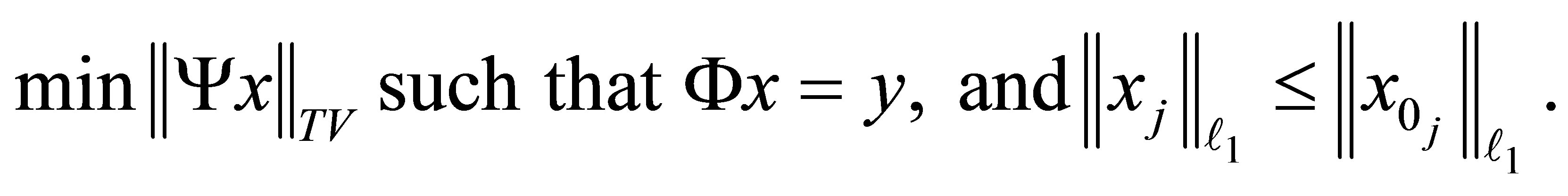(4)

The -constraints restrict the locations where the large wavelet coefficients can appear, assuming the -values of each subband

are known. In their experiments, random Fourier matrices were applied to the wavelet coefficients of the images. The number of measurements were taken to be 15%, 23%, 30%, and 38% of the total number of pixels, i.e., 256 × 256. It was shown that the recovery from 3k to 5k random projections is comparable to the best k-term wavelet approximation [13].

The main results in [12] by Candès, Romberg and Tao are that the standard compressed sensing is able to stably recover sparse as well as compressible signals from noisy measurements. For the latter, if k is chosen such that and in (1) satisfy, the error bound for compressible signals with noise in the measurements is

(5)

where is the true signal, is the recovered signal, is the best k-term approximation of, μ is any perturbation, and constants and depend on. It is stated (Theorem 2, [12]) that minimization stably recovers the -largest entries. As the authors point out, this is a deterministic statement, i.e., there is no probability of failure. Their experiments on both 1D and 2D compressible signals with noise added to measurements confirm this theoretical result. It is also observed in their experiments that if the noise is Gaussian with small standard deviation, then the recovery error is dominated by the approximation error, i.e., by the last term in (5).

Even though the above methods and results deal with non-sparse compressible signals they are not deterministic in the sense that the measurements are obtained via random projections. In practice, it is beneficial to use deterministic sensing matrices that are pre-determined in order to save computation time and memory. Work in this direction was done by DeVore [14], then followed by a few others. However, the recovery results were far inferior compared to that obtained by traditional random sensing. Recently, another deterministic compressed sensing method (mainly applicable for 1D signals) was proposed by Applebaum, Howard, Searle, and Calderbank [15] by using the chirp transform to create the sensing matrix. In their experiments (Figures 2 and 3 in [15]), the full pass chirp decode algorithm results in smaller reconstruction error than using Gaussian random matrices with matching pursuit. They have also shown empirically (see Figure 4 in [15]) that these two methods are comparable when there is noise in the measurements. The reconstruction algorithm is good for 1D signals but in experiments given in [15] the 1D signals are of size or 67² only, much smaller than the size encountered for 2D signals, such as images. A similar reconstruction algorithm was also proposed for a sensing matrix made from Reed-Muller sequences [16]. In [3], we proposed new reconstruction algorithms for deterministic sensing matrices made from chirp and Reed-Muller sequences that are suitable for 2D images.

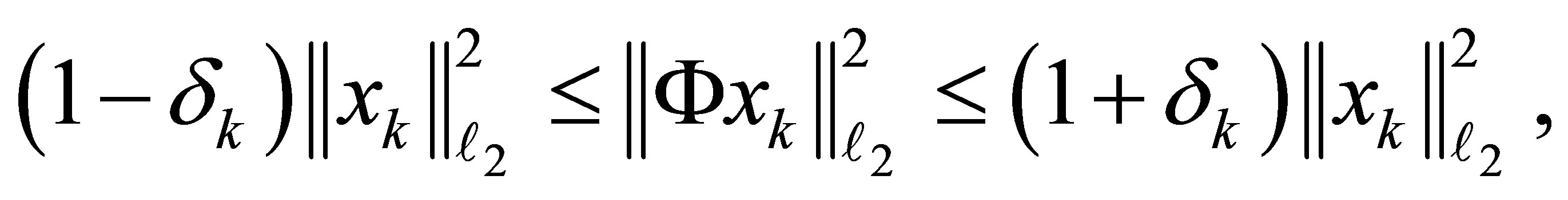
The advantage of using deterministic matrices for compressed sensing is that reconstruction can be very efficient [15,16]. The fast reconstruction algorithm [15-17] is called the Quadratic Reconstruction Algorithm. This algorithm takes advantage of the multivariable quadratic functions that appear as exponents of the entries in the sensing matrix, and therefore, only requires vector-vector multiplication instead of matrix-vector multiplication required in Basis and Matching Pursuit algorithms that are used for reconstructions with random sensing matrices. In [17], Calderbank, Howard and Jafarpour set forth criteria on Φ that ensure a high probability that the mapping taking the k-sparse signal vector to the measurement vector y is injective, assuming a uniform probability distribution on the unit-magnitude k-sparse vectors in. They say that Φ has the Statistical Restricted Isometry Property (StRIP) with respect to parameters and δ if

(6)

holds with probability exceeding when is assumed to be uniformly distributed among k-sparse vectors in of some fixed norm (e.g., unit norm). They show that such deterministic sensing matrices satisfying StRIP can be constructed by chirps, Reed-Muller (RM) sequences, and BCH codes, as done in [15-17]. In the presence of noise, if Φ satisfies the StRIP property with parameters and δ, the reconstruction error due to the Quadratic Reconstruction Algorithm is given by

(7)

where is the true signal, is the recovered signal, is the best k-term approximation of, and μ is the measurement noise from a Gaussian distribution, see [17]. As mentioned there, this bound is tighter than bounds obtained by using random ensembles [12] and expanderbased methods [18]. While the Quadratic Reconstruction Algorithm [15,16] is shown to accurately reconstruct 1D sparse signals with nonzero locations chosen uniformly at random, from a small number of measurements, it does not work when it is directly applied to 2D signals, like images. This is because the locations of the nonzero coefficients, usually in the wavelet domain, are not distributed uniformly. Our proposed algorithm [3] takes this into account and we have shown that it outperforms a standard compressed sensing method, which takes random noiselet measurements and uses minimization for reconstruction, for example, see [19].

Authors in [17] also derived that the deterministic sensing matrices are resilient to noise. Suppose the noise comes from the measurements, say, where μ are iid complex Gaussian random variables with zero mean and variance. Suppose Φ satisfies

(8)

with probability exceeding. Then, for,

(9)

with probability exceeding, where

(10)

Therefore, we see that the noisy measurement is bounded in (9) by the signal in a similar way as the inequality (8) in the StRIP property.

Now, suppose that the noise comes from the signal, say, where μ is a complex, multivariate, Gaussian distributed noise with zero mean and covariance. In this case, the estimates given in (9) can still be applied. The covariance of the measurement vector is

For deterministic matrices, and this gives

The factor that appears in is not present in making the measurement variance in this case larger than the source noise variance. This means that noise coming from the signal is harder to deal with than noise coming from the measurements.

One important and desirable task in reconstruction of signals via deterministic compressed sensing is to reconstruct signals efficiently. Moreover, such reconstruction should be stable under noise and also work when the signal is non-sparse. In this paper, we discuss the stability and robustness of the algorithms we introduced in [3]. We show that these algorithms are stable for non-sparse (compressible) signals and robust under various types of noise. In addition, we also indicate how, when using the sensing matrix composed from Reed-Muller sequences, the algorithms in [3] may be modified to efficiently handle excessively large images or large 2D signals.

This paper is structured as follows: in Section 2, we review our reconstruction algorithm of [3] and comment on how to incorporate properties of the Reed-Muller sequences so that the algorithm can handle images of size much larger than considered so far. Then we discuss how to choose the proper wavelet domain and the level of decomposition of the image under the chosen wavelet basis. In Section 3, we discuss the stability and robustness under noise and for non-sparse signals. Finally, Section 4 contains the discussion of the results.

2. Choosing a Suitable Sparsifying Domain

We address the issue of choosing a suitable sparsifying domain for images, since the compressed sensing theory is based on the fact that the signal is sparse. Wavelets are commonly used for 2D images, but the choice of the specific wavelet to be used is not usually discussed much. In the next few subsections, we first review the fast reconstruction algorithm for 2D signals including comments on modifying the Reed-Muller sensing case based on certain properties of the Reed-Muller sequences. Then we discuss how to choose a suitable Daubechies DN wavelet basis and the optimal level of decomposition. The images used in this work are shown in Figure 1, where 1) is a 512 × 512 MR image of brain, 2) is a 512 × 512 MR angiogram image, and 3) is a natural image of 1024 × 1024 resolution, which we refer to as the man image.

2.1. Reconstruction Algorithm for Deterministic Sensing Matrices

We start with a discussion of deterministic compressed sensing using chirps, i.e., frequency modulated discrete sinusoids. Our reconstruction algorithm using ReedMuller sequences is similar and is briefly discussed here as well. The detailed reconstruction technique for both can be found in [3].

2.1.1. Compressed Sensing with Chirps

A discrete chirp of length n with chirp rate r and base frequency m has the form

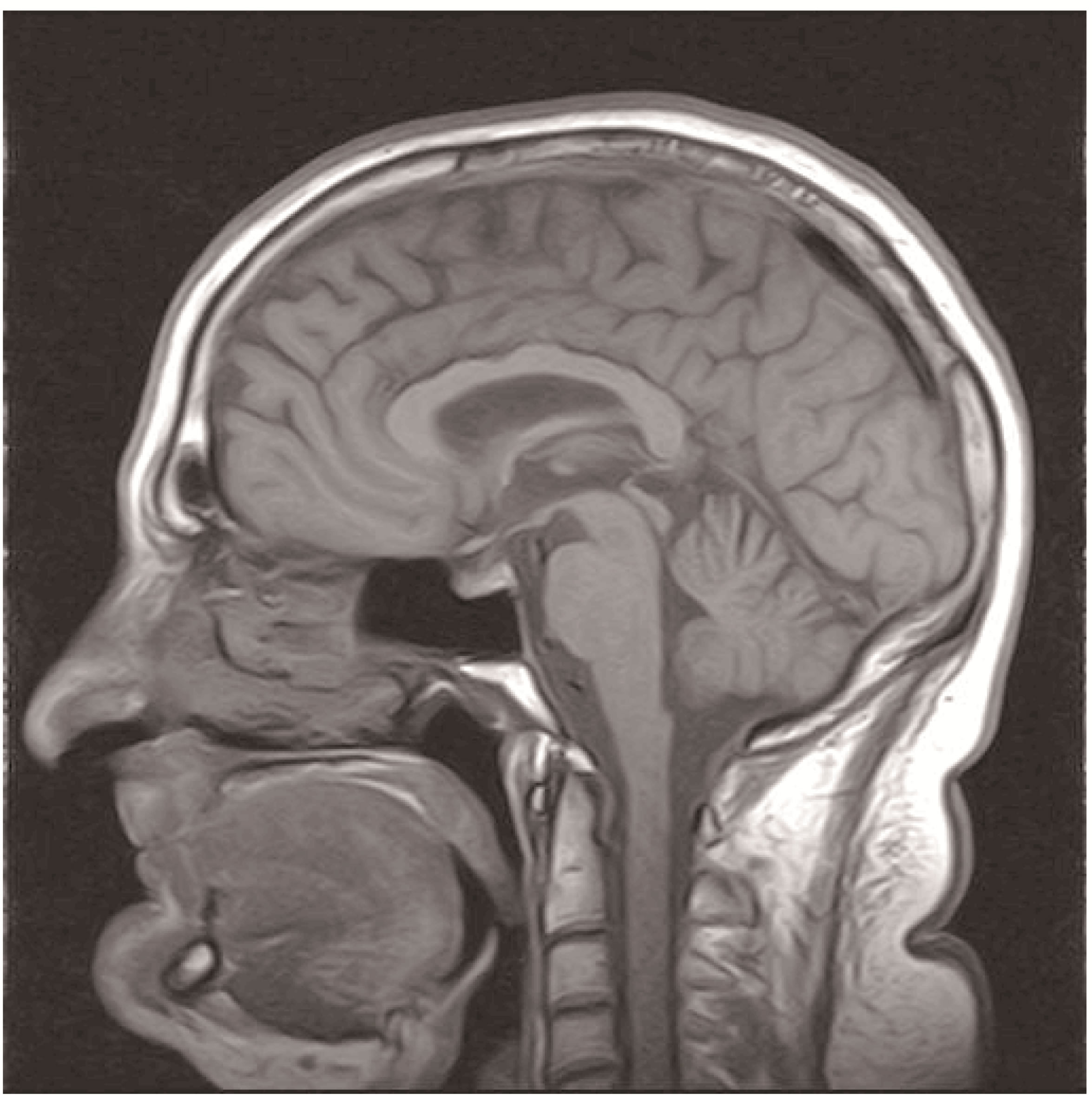
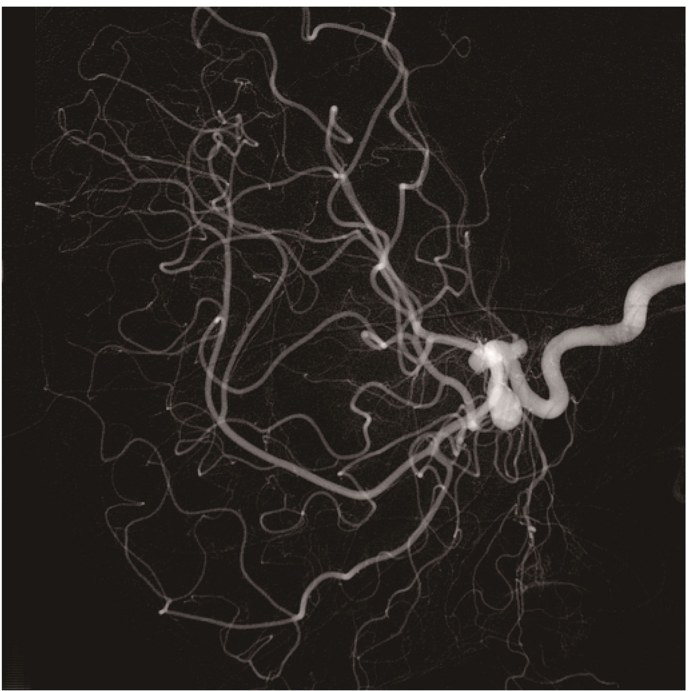
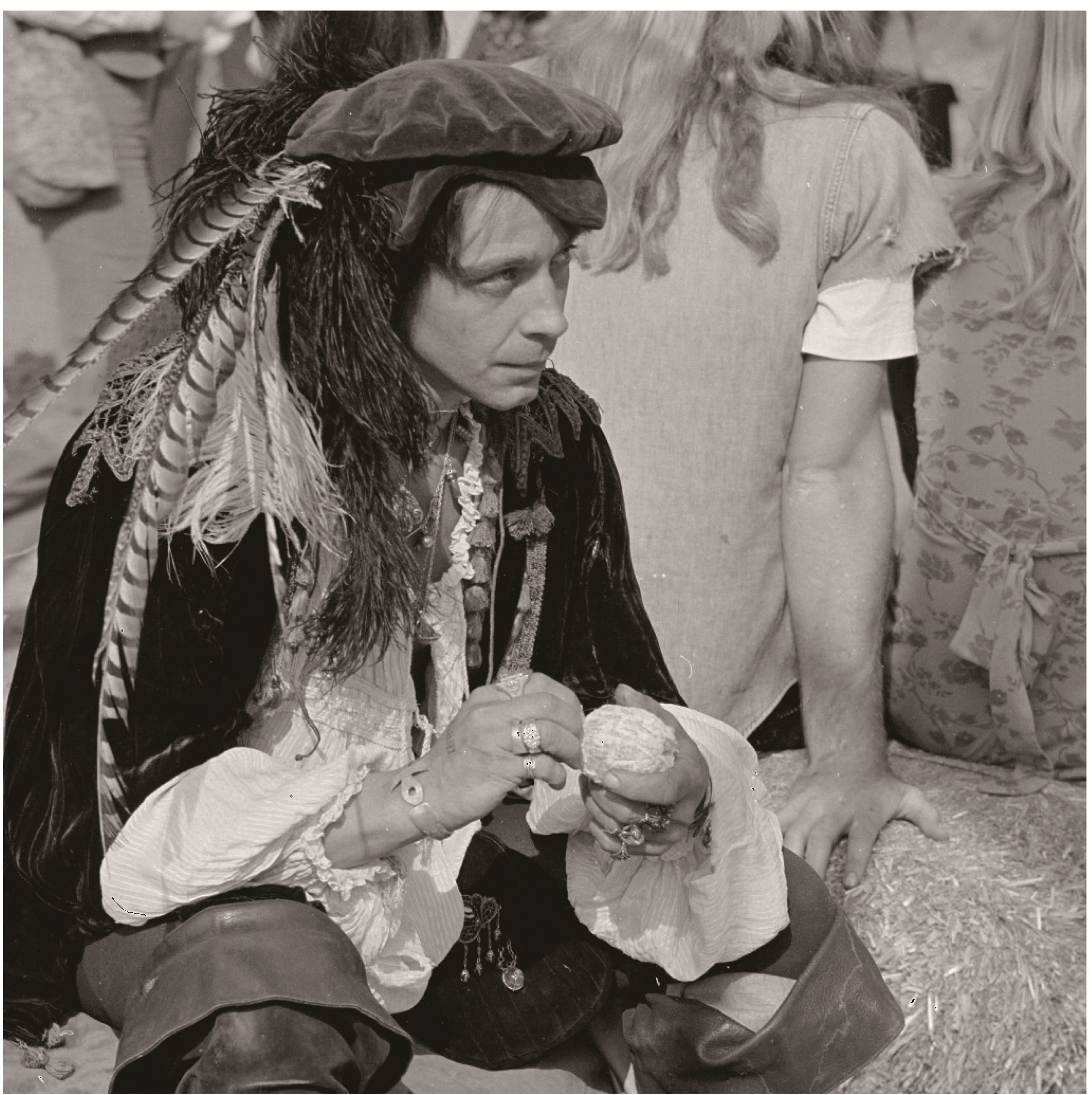
(a) brain                             (b) vessel                              (c) man

Figure 1. 2D images used in this paper.

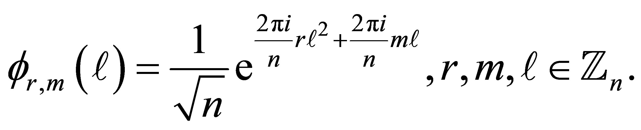(11)

Note that the coefficient is present in order for the vector to have a unit norm. For a fixed n, there are n² possible pairs (r, m). The full chirp sensing matrix Φ thus has size n × n² and can be written as

(12)

Each is an n × n matrix with columns given by chirp signals having a fixed chirp rate with base frequency m varying from 0 to n − 1. The chirp rate r also varies from 0 to n − 1. Therefore, column of is a discrete chirp with chirp rate r and base frequency m.

Example 2.1. Let Then

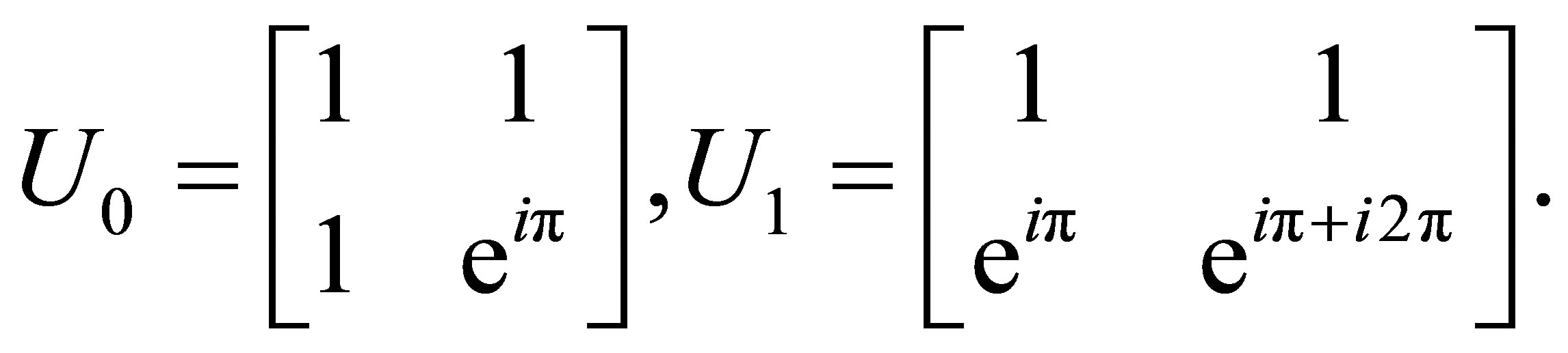
The 2 × 4 sensing matrix is then given by

Note that U₀, the n × n matrix corresponding to chirp rate is the Discrete Fourier Transform (DFT) matrix. The Fast Fourier Transform (FFT), which implements the DFT, is used in the algorithm for recovering a sparse signal from chirp measurements, see Section 2.1.5.

2.1.2. The Chirp Sensing Matrix for 2D Signals

Despite the success in accurate reconstruction of very sparse one-dimensional (1D) signals with the algorithm described in [16], applying it to real two-dimensional (2D) images is impractical. This is because, in general, real images are not as sparse in any transform domain as the one-dimensional signals used in [15] or [16].

A good approximation of a 256 × 256 pixel image is typically obtained by retaining the largest 10% wavelet coefficients in some suitably chosen wavelet domain. In particular, many medical images are well approximated by transform coding using 10% - 20% of their wavelet coefficients, but begin to show appreciable degradation as the percentage of coefficients retained falls below these levels. However, a 256 × 256 image with 10% sparsity has 6554 nonzero coefficients, which is much larger than the sparsity considered for the 1D signals in [15,16]. A rule of thumb, see [20, Theorem 1], for the number of measurements in the standard compressed sensing using the Gaussian random matrices with minimization is given by

(13)

This rule guarantees successful reconstruction with high probability if the number of measurements n is large compared to the sparsity and signal size. Using (13) in the above example, at least 22,672 measurements are needed for the correct reconstruction. The ratio is 2.89, and this implies that roughly only three chirp rates are needed to form the sensing matrix.

As explained above, due to the nature of sparsity of images and the rule of thumb (13), a few sub-matrices of can be used to make the sensing matrix, with the ratio for 10%-sparse images. In practice, a larger ratio can be used, such as 4 for 10%-sparse images, which will be analyzed later. Consequently, there is more freedom in the choice of the chirp rates r when constructing the sensing matrix.

The inner product of any pair of distinct chirp vectors is as follows:

(14)

Therefore, a submatrix should use as few chirp rates as possible and the choice of the chirp rates can be arbitrary. For example, the submatrix can be

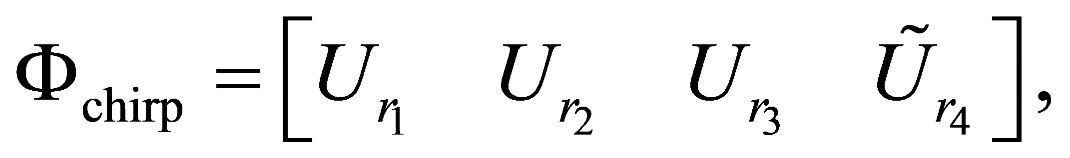(15)

where and denotes a submatrix of so that the number of columns of matches the signal size. When only the first J submatrices are used to form the sensing matrix, it follows from an argument given by Alltop ([21], Section 4) that n need not necessarily be prime. Rather, the crucial condition for unique identification of the chirp rate r_t in the reconstruction algorithm is that the smallest prime divisor of n is greater than J. For instance, the sensing matrix for a 256 × 256 (N = 65,536) image may be taken to be of size n × N = 16,385 × 65,536. Note that 16,385 = 5 × 29 × 113 is closest to and larger than 25% × 65,536 = 16,384 whose smallest prime divisor is greater than 4. Here, the 25% ratio comes from the fact that four chirp rates are used. In this example, is of size 16,385 × 16,381 and can be without the last four columns.

2.1.3. Reed-Muller Sequences in Deterministic Compressed Sensing

The set of real valued second-order Reed-Muller (RM) codes or sequences with length is parameterized by p × p binary symmetric matrices P and binary p-vectors. In terms of these parameters, a second-order RM code is given by

(16)

In analogy with the chirps, the vector b in the linear term of (16) and the matrix P in the quadratic term may be regarded as the “frequency” and “chirp rate” of the code, respectively. In the expression (16), indexes the components of the code. So, for given parameters P and b, the code is a vector of length. These vectors will serve as the columns of the sensing matrix. In addition, during implementation, P is taken to be zero on its main diagonal to ensure that the codes generated are real valued. This implies that the components of these codes are all ±1.

Example 2.2. Let p = 2 then

and There are

zero diagonal symmetric matrices of size 2 × 2. These are

and

Set Then if we get for

Similarly, for other values of a in, one gets

The vector will be one of the columns of the sensing matrix.

In general, the compressed sensing matrix proposed in [16] has the form

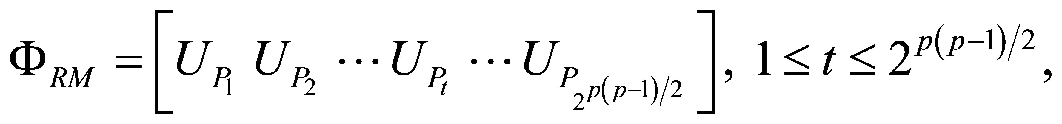(17)

where each is a orthogonal matrix whose columns are with b going through all binary p-vectors. In addition, each is multiplied with a phase factor, where is the Hamming weight of b, i.e., the number of ones in b. The extra phase factor ensures that the total number of plus and minus signs of the inner products of any two columns are the same. For convenience, is chosen to be the zero matrix, and therefore, without the phase factor, is a Hadamard matrix up to a scaling [22]. Consequently, multiplication by is the Walsh-Hadamard transform (DHT) which, up to a scaling, is its own inverse [22]. In the reconstruction of a sparse signal using the ReedMuller sensing matrix the algorithm uses the DHT, see Section 2.1.5. This is analogous to the DFT that is used with the chirp sensing matrix.

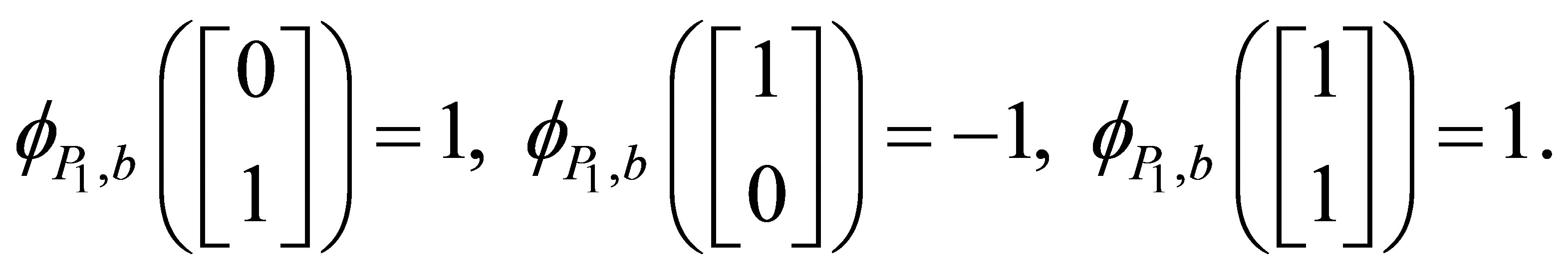
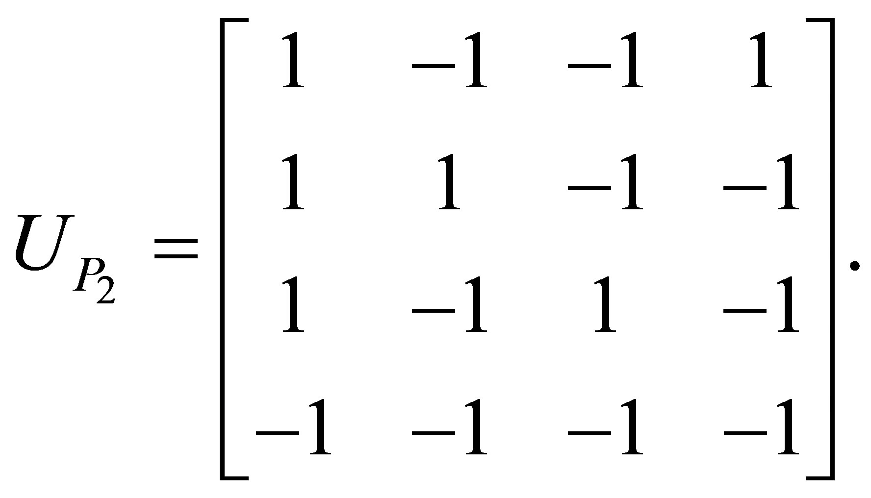
Example 2.3. In Example 2.2,

In this case, the first column corresponds to

the second column corresponds to (as shown in Example 2.2), and so on. Similarly, for the matrix we get

Together, we get the Reed-Muller sensing matrix, for p = 2, as

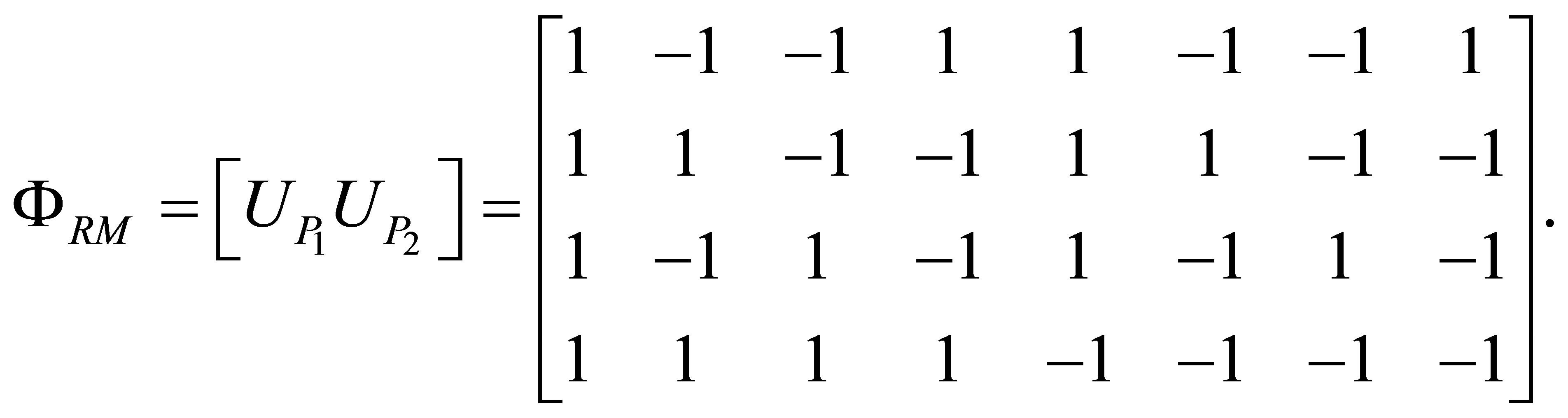
As noted earlier, the vector b in the linear term of (16) and the matrix P in the quadratic term may be regarded as the binary “frequency” and “chirp rate” of the code, respectively. There are such P matrices with zero-diagonal, so the maximum size of the RM sensing matrix in (17) is. For a given P, codes are obtained by varying b, yielding the columns of a orthogonal matrix

The Delsarte-Goethals set is the binary vector space of binary symmetric matrices with the property that the difference between any two distinct matrices has rank greater than or equal to [23]. Evidently, these sets are nested

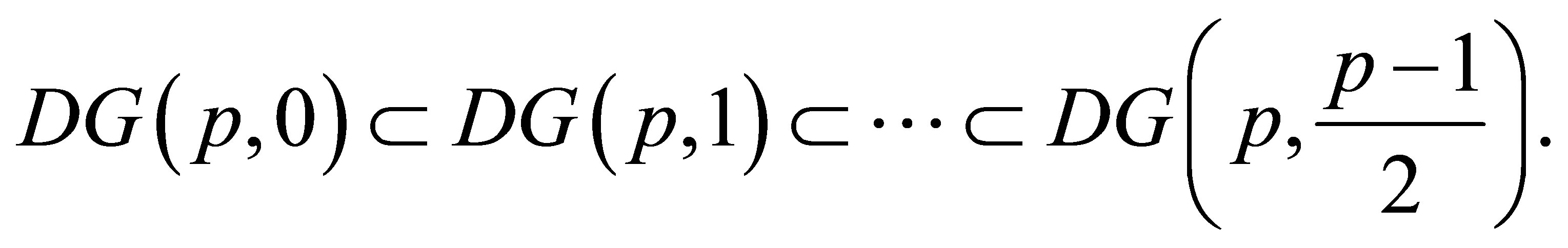(18)

Example 2.4. Let Then DG(3,0), consisting of matrices whose differences have rank at least 3, is spanned by the set [24]

The set DG(3,1), consisting of matrices whose differences have rank at least 3 − 2 = 1 is spanned by [24]

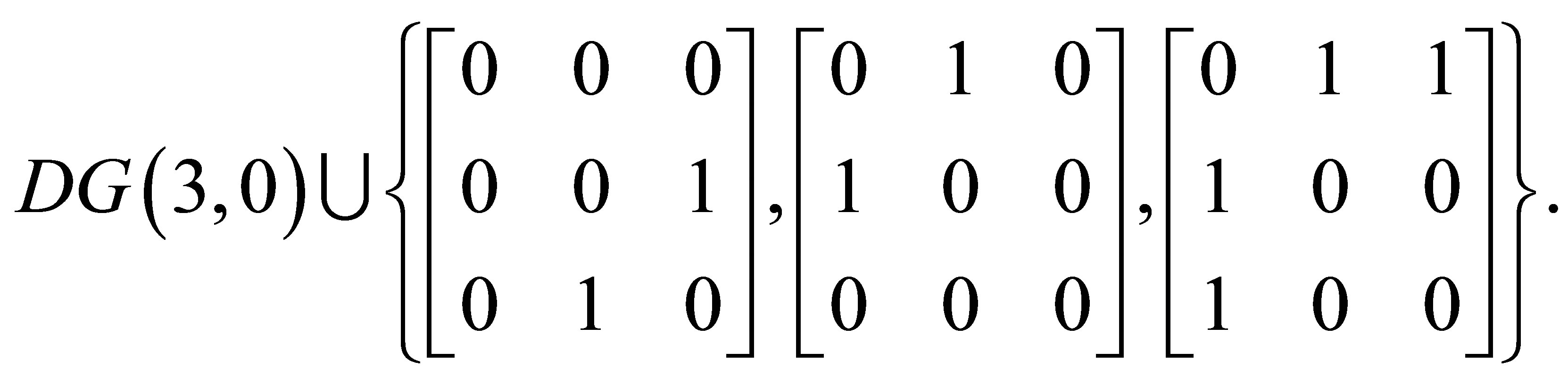
Note that these 6 matrices generate all the 2⁶ binary symmetric matrices of size 3 × 3.

The set of all P matrices that reside in DG(p,0), is called the Kerdock set. This means that the difference between any two distinct matrices in the Kerdock set has full rank. The Reed-Muller codes made from the matrices P in the Kerdock set produces the Kerdock codes [25]. Two distinct Kerdock codes, normalized to unit length, have inner product modulus that is either zero (if they correspond to the same P) or (if they correspond to distinct Ps). More generally,

(19)

where. So, if the domain of P is DG(p, q), the set of possible inner product modulus values for distinct normalized codes is.

Allowing P to range over all of, (16) gives the full set of second-order RM codes.

Defining and, a k-sparse signal yields a measurement, which is the superposition of k RM functions

(20)

In (20), z_t are used instead of x in order to only write the nonzero terms, and P_t and b_t may individually repeat in the equation.

2.1.4. The Reed-Muller Sensing Matrix for 2D Signals

When forming a sensing matrix from submatrices of the RM matrix given in (17), the choice of the submatrix cannot be arbitrary. The inner product of two columns of, one taken from and another from, , is given by (19) with. If q = p, the inner product is always, which is smaller than the inner product in other cases, q < p. Since the nonzero locations of the signal are unknown, it is desirable that the inner products between any two columns are as small as possible, thus making the columns of the resulting sensing matrix close to orthogonal. Taking q = p, and thus drawing P matrices only from DG(p,0), (i.e., the Kerdock set) gives the best situation. For a given p, there are zero-diagonal matrices in the Kerdock set [24]. A sensing matrix can be constructed in the form

(21)

where P₁, P₂, P₃, and P₄ are matrices from the Kerdock set. The idea behind choosing four P matrices or chirp rates is the same as that discussed in Section 2.1.2 for the chirp sensing matrix. For example, the sensing matrix for a 256 × 256 (N = 2¹⁶) image with 10% sparsity is of size n × N = 2¹⁴ ×2¹⁶ which means that only 25% of the signal entries are sampled. Note that for images with sparsity much smaller than 10%, fewer measurements are needed, and therefore, more P matrices can be used, since the ratio becomes larger.

2.1.5. The Reconstruction Algorithm

Here we outline the reconstruction algorithm. For more details, we refer the reader to [3].

Input: y and

Output:

1) Approximation: Perform hard-thresholding to obtain a set of nonzero locations, denoted by. Let be a submatrix of restricted on the set. Then, the initial approximation is and the residual is obtained by.

2) Detection¹: From

where is the first column of, update

.

Let.

3) Least Squares:

4) Define. Repeat 2.-4. until is sufficiently small.

If all the non-zero terms are caught by the set then the precision of reconstruction is dependent on the LSQR algorithm [26] that is used in step 3) above.

2.2. Using the Hierarchy of the Delsarte-Goethals (DG) Sets for Larger Signals

So far while using the RM sensing matrix the size of the images was such that it was possible to pick all the P matrices, needed to construct the sensing matrix, from the Kerdock set. Sometimes one has to deal with signals whose sizes are such that the required sensing matrix has to be larger than what can be obtained only from the Kerdock set. Then we have to move on to P matrices from the DG sets that do not have the full rank property of the Kerdock matrices. This leads us to look at the rank and other properties, see, for example, (18), of matrices from the DG sets as described in Section 2.1.3. In this case some assumptions on the signal are useful. Compressed sensing for signals with prior information has been addressed by other authors [27-30]. These authors design appropriate reconstruction algorithm but not sensing matrices as we do here.

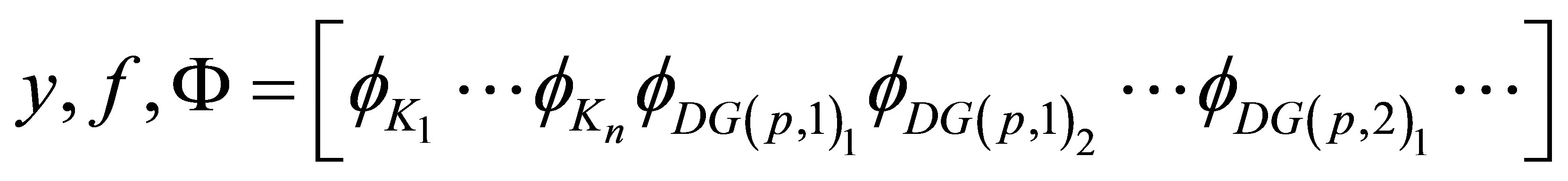
We assume that there is some a priori knowledge of the behavior of the signal coefficients. Let us suppose that the signal is sparse and the coefficients of the signal (with respect to some sparsity domain, for example, some wavelet basis) follow a decay pattern. This means that for each location in the signal we know the probability of having a non-zero value. In this case the sensing matrix from the second order Reed-Muller sequences can be constructed in the following way. We start assigning vectors generated from P matrices in the Kerdock or DG(p,0) set to the columns of the sensing matrix that correspond to the signal locations that are most likely to be non-empty. Once the Kerdock set is exhausted we take vectors that come from DG(p,1), DG(p,2), and so on following the hierarchy given in (18). Alternatively, without any loss of generality, one can assume that the signal elements are arranged in ascending order. Then the columns of the sensing matrix appear in the DG order, i.e., the columns from the Kerdock set come first, followed by the DG(p,1) and so on. So

This is outlined in the following algorithm. Note that in the algorithm given below, f is the probability density function of the nonzero (or active) locations. It is assumed to be a decreasing function, which corresponds to the design of the DG matrix.

Input:

Output:

Initially, the residual.

1) Detection: From

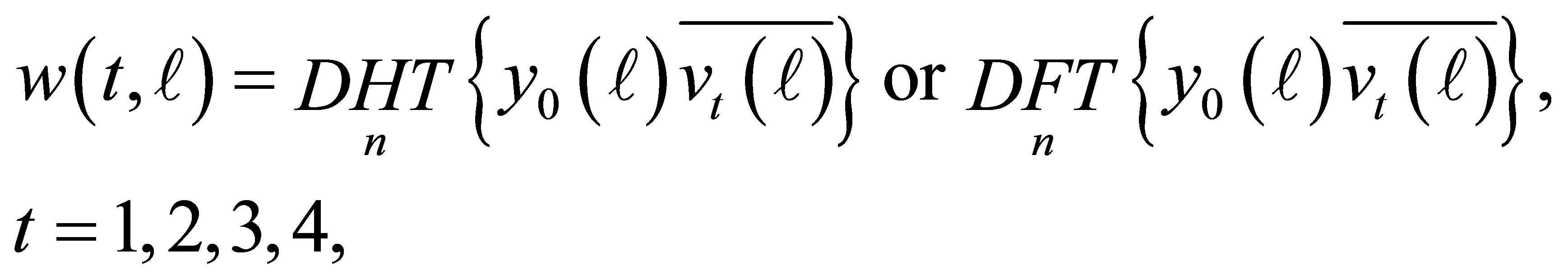
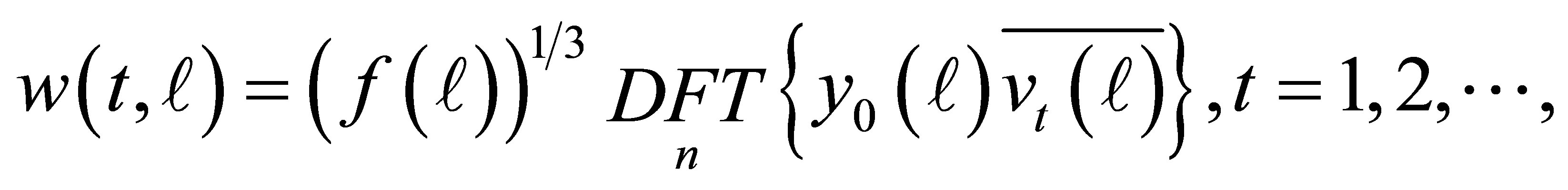where DFT is DHT in the RM case and is the first column of, update

. Let.

2) Least Squares: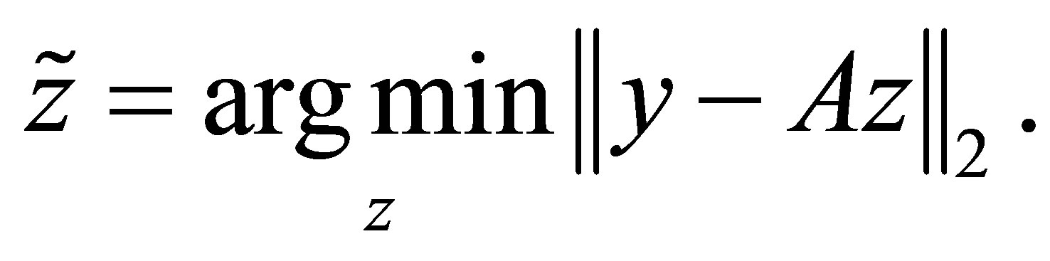

3) Define. Repeat 1)-3) until is sufficiently small.

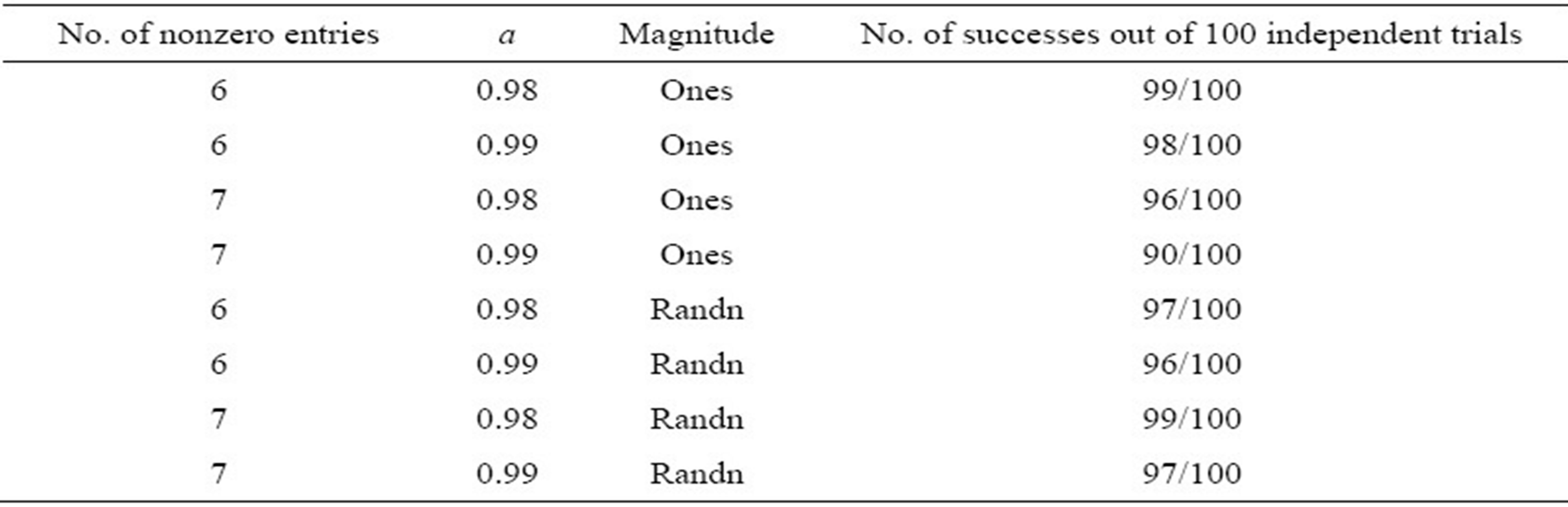
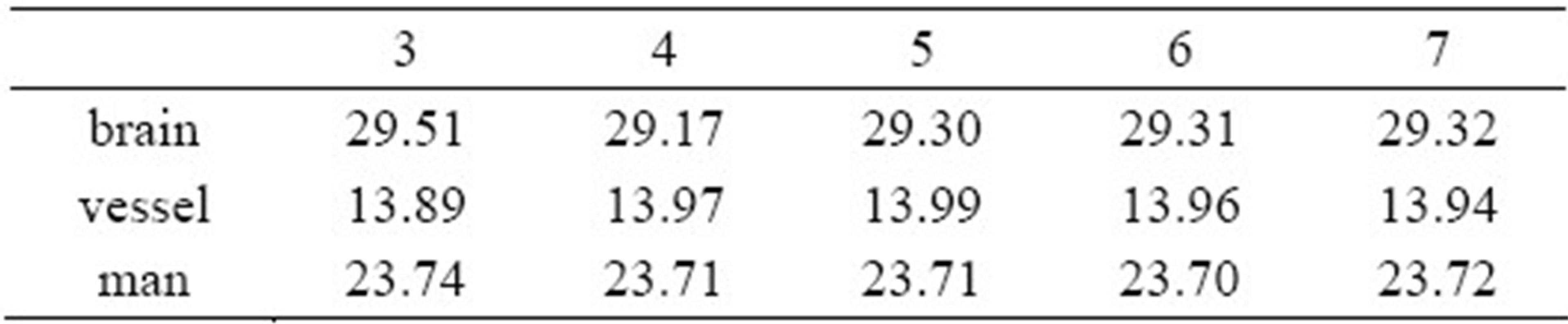
Some preliminary results have been obtained by using the above method and are given in Table 1. According to the rule of thumb, as given in (13), if we have a signal of size 2²¹ and we wish to recover this using 2⁶ measurements, then the sparsity should satisfy However, our results in Table 1 indicate that with our algorithm, using the DG order, we are able to recover signals with sparsity greater than 3. This is part of ongoing and future work.

2.3. Choosing the Best Daubechies Wavelet Basis

It is commonly believed that the Haar wavelet (D2) works best for 2D images in compressed sensing. This is because many images chosen for experiments are relatively small, i.e., at most 128 × 128. In this paper, we are interested in higher-resolution images, such as 512 × 512 and 1024 × 1024. The degree of smoothness in an image loosely determines the support width of polynomials. For an image scene, if the image resolution is large, the de-

Table 1. The density function used is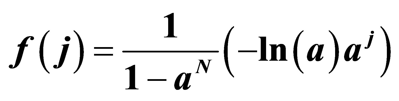. Signal size is N = 2²¹, sparsity k = 6, 7, measurement size or no. of rows of the sensing matrix = n = 2⁶ = 64. The magnitude of the signal entries are either ones or randn (normally distributed pseudorandom).

gree of smoothness becomes large. Therefore, an appropriate support width should be large.

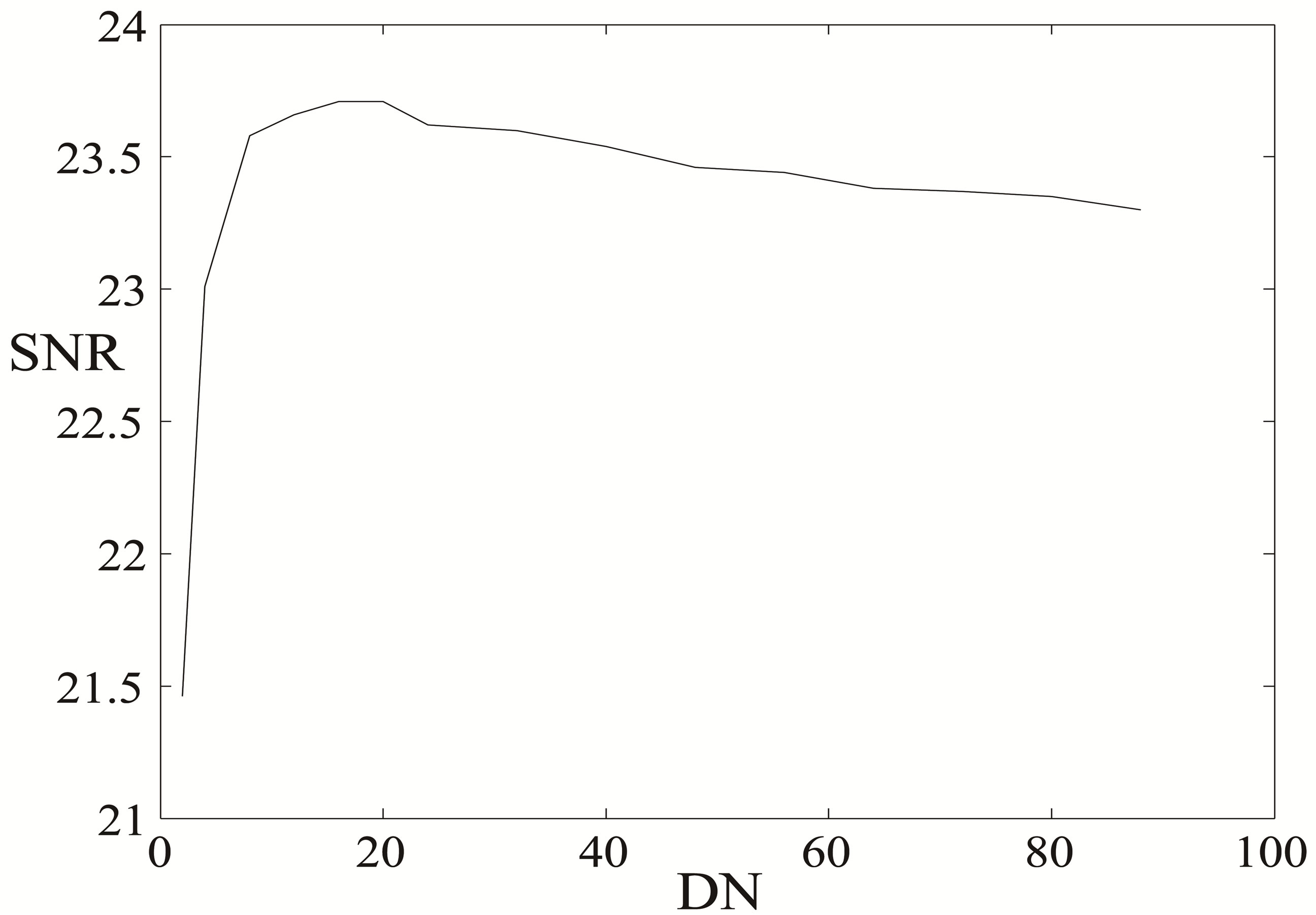
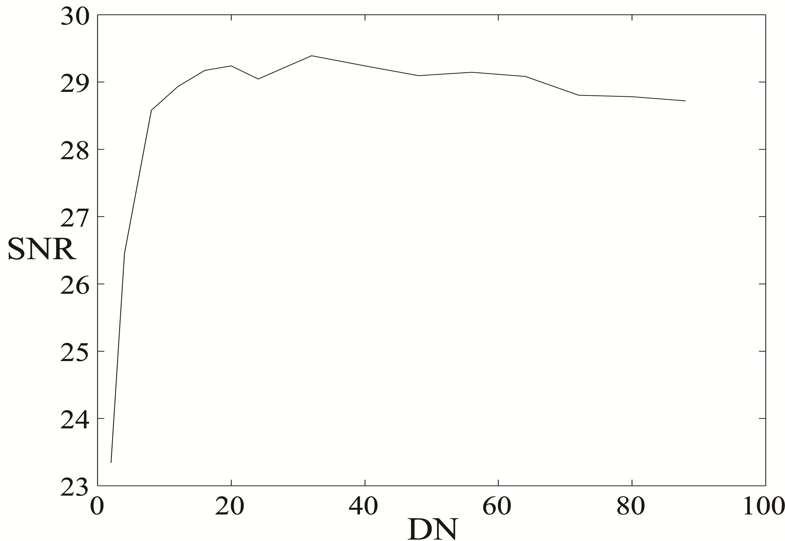
Figure 2 shows experiments of chirp compressed sensing using different Daubechies wavelet transforms. The vertical axis is the reconstruction SNR in dB using chirp compressed sensing. The horizontal axis shows which Daubechies wavelet DN (or in Matlab) is used as the sparsifying domain. The level of decompositions is fixed here and is equal to 4 levels (see explanation about the levels in Section 2.2). In particular, D2 (or db1 in Matlab) is the Haar wavelet. The 2D images are not sparsified. The number of measurements taken is 25% of the number of pixels. In all three plots, the reconstruction SNR is optimal around D16. More strictly, the largest reconstruction SNR is within 0.5 dB from the reconstruction error at D16. The decay is faster in the vessel image (b) than in the images (a) and (c), since the vessel image is sharper than the brain and man images and contains more edges. See Table A1 in Appendix for the precise values. Therefore, we suggest using D16 wavelet basis in deterministic compressed sensing. In particular, instead of the Haar basis our results are obtained using D16 basis.

2.4. Number of Levels for Wavelet Decomposition

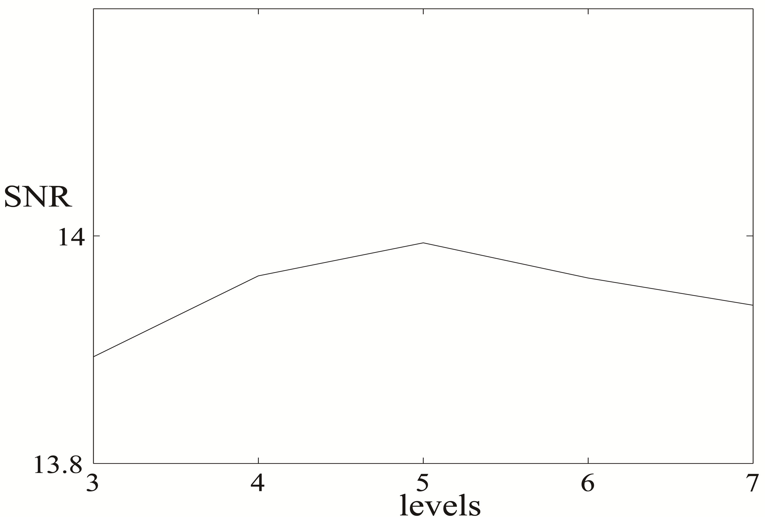
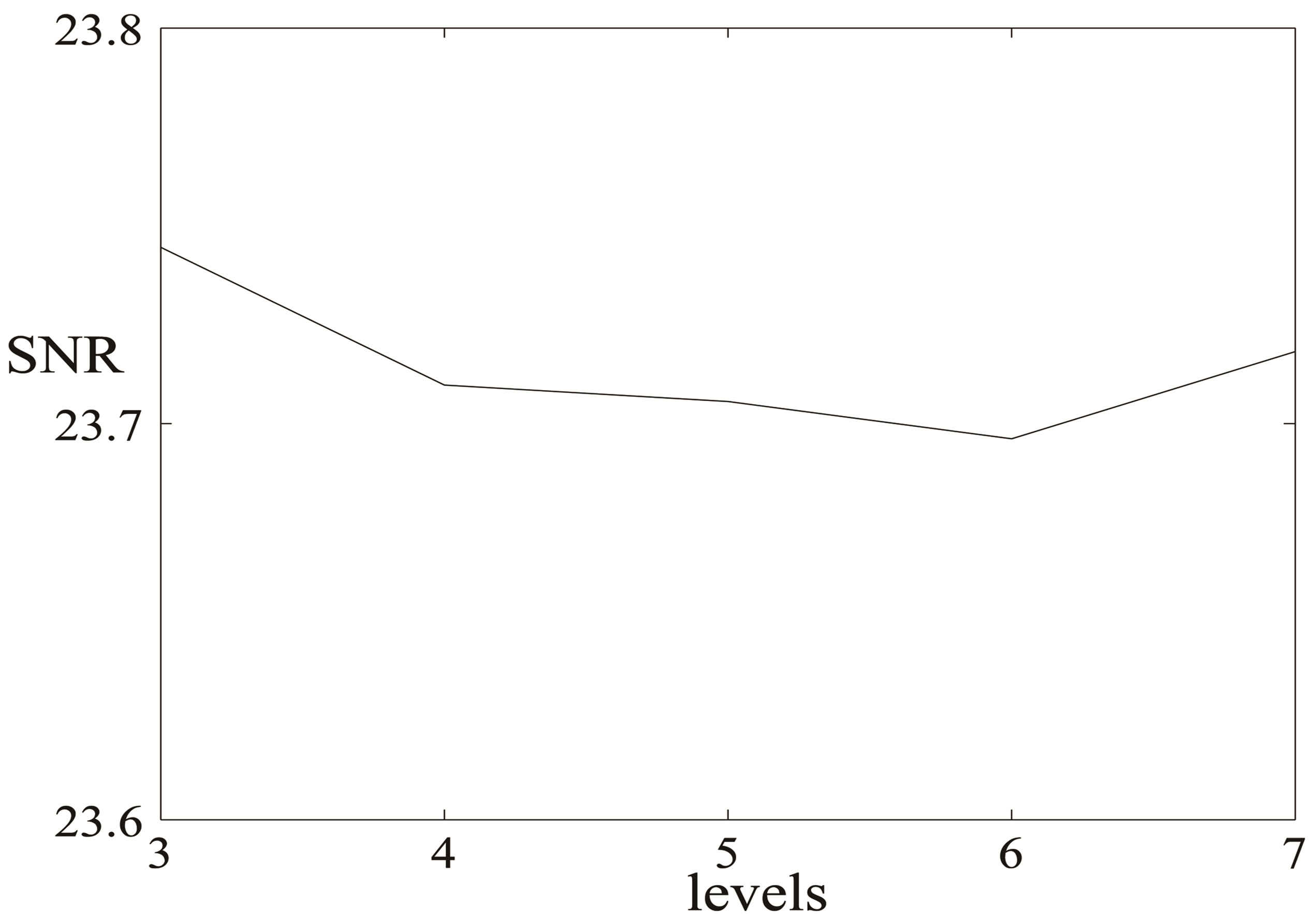
In this subsection we investigate how many levels of decomposition should be used in the reconstruction of large images. Figure 3 shows experiments of chirp compressed sensing using D16 with different levels of decomposition. The vertical axis is the reconstruction SNR in dB using chirp compressed sensing. The horizontal axis is the number of levels. In (a) and (c), 3 levels give the best reconstruction SNR. However, we observe that the sparsified images with 3 levels lost a lot more details than with higher levels, when compared to the original un-sparsified images. Therefore, we do not choose 3 levels. The reconstruction SNR from level 4 to 7 is within 0.1 dB range. For experiments in the next section, we thus choose 4 levels. See Table A2 in Appendix for the precise values.

3. Stability of the Deterministic Compressed Sensing Algorithms

By the observations in the previous section, we use Daubechies D16 with 4 levels of wavelet decomposition in all of the following experiments. To study the stability of deterministic compressed sensing using chirp and Reed-Muller sequences for 2D images under noise, we consider five cases. In the first three cases, the noise is in the sparse signal, before the transform Φ is taken. In the last two cases, the noise is added after the transform. In what follows we choose the noise to be iid Gaussian with mean zero and variance. The following are the cases:

1) The 2D images are sparsified with pre-defined sparsity in the wavelet domain. The wavelet coefficients is k-sparse and there is a noise in the wavelet domain. The measurement is

(22)

2) The wavelet coefficients, denoted by x₀, is not sparsified, but assumed to be compressible. The noise is again in the wavelet domain. The measurement is

(23)

3) The wavelet coefficients x_k is k-sparse and the noise in the wavelet domain, is only non-zero outside the support of. Here stands for the complement locations of the non-zero wavelet coefficients, i.e., the noise is added to the zero wavelet coefficients. Therefore, the nonzero coefficients of the signal are not perturbed. The measurement is

(a) brain                                 (b) vessel                                (c) man

Figure 2. Reconstruction SNR (in dB) of chirp compressed sensing with different Daubechies wavelet DN (or in Matlab) and 4 levels of wavelet decomposition. The 2D images from Figure 1 are not sparsified. The number of measurements taken is 25% of the number of pixels.

(a) brain                                (b) vessel                               (c) man

Figure 3. Reconstruction SNR (in dB) of chirp compressed sensing with Daubechies D16 wavelet and different number of levels of wavelet decomposition. The 2D images are not sparsified. The number of measurements taken is 25% of the number of pixels.

(24)

4) Noise occurs at the step of measurements and is added after the signal is transformed by the CS matrix Φ:

(25)

5) Noise occurs at the step of measurements and is added after the compressible non-sparse signal x₀ is transformed by Φ:

(26)

We test our algorithm on 3 images, see Figure 1, which we refer to as brain, vessel, and man. The first two are typical MRI images used in the medical community, and the third is a high resolution natural image. We reconstruct these images using chirp and Reed-Muller sensing matrices and compare with the reconstruction by noiselets (for example, see [31]). The noiselet method takes random noiselet measurements and then reconstructs by minimization whereas our chirp and ReedMuller algorithms use deterministic measurements and the reconstruction is by a least squares method.

The reconstruction error is defined as:

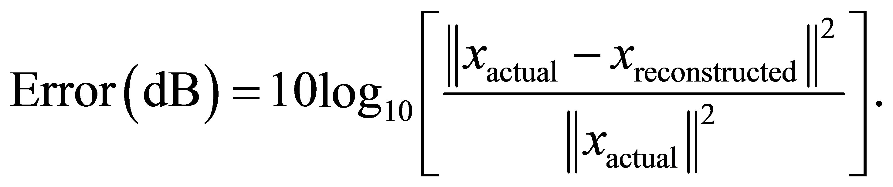
The negative of the above error is known as the signal-to-noise ratio (SNR). Tables 2-6 show the reconstructed SNR of measurements taken according to (22)- (26), respectively. Several noise levels were chosen for the experiment; and specifically, the standard deviation σ of Gaussian noise with zero mean are σ = 0, 0.01, 0.05, 0.1 and 0.2. These values are chosen for comparison purposes, for example, with Tables 1 and 2 in [12].

For Tables 2-4, the third columns are the SNR of the noisy images compared to the images before noise is added to the wavelet coefficients. If noise is present in the signal, all reconstructed SNR are smaller than the reference SNR via noiselet measurements and minimization. The reconstructed SNR by chirp has the highest value (best) in all cases and stays very close to the reference SNR. The reconstructed SNR by RM is higher than noiselets when the noise level is small.

When the noise level is large, it seems that the noiseTable 2. The 2D images are first sparsified in the domain of Daubechies wavelet D16 (db8 in Matlab) with 4 levels of decomposition. The image, its size, and the pre-determined sparsity are shown in the first column. Gaussian noise with zero mean and variance σ² (or standard deviation σ) is added to the wavelet coefficients of the sparsified image; see (22). The third column shows the SNR in dB compared to the noise-free sparsified image. Columns 4-6 show the reconstruction SNR in dB using noiselets, chirp, and Reed-Muller CS algorithms, respectively. The number of measurements taken is 25% of the number of pixels.

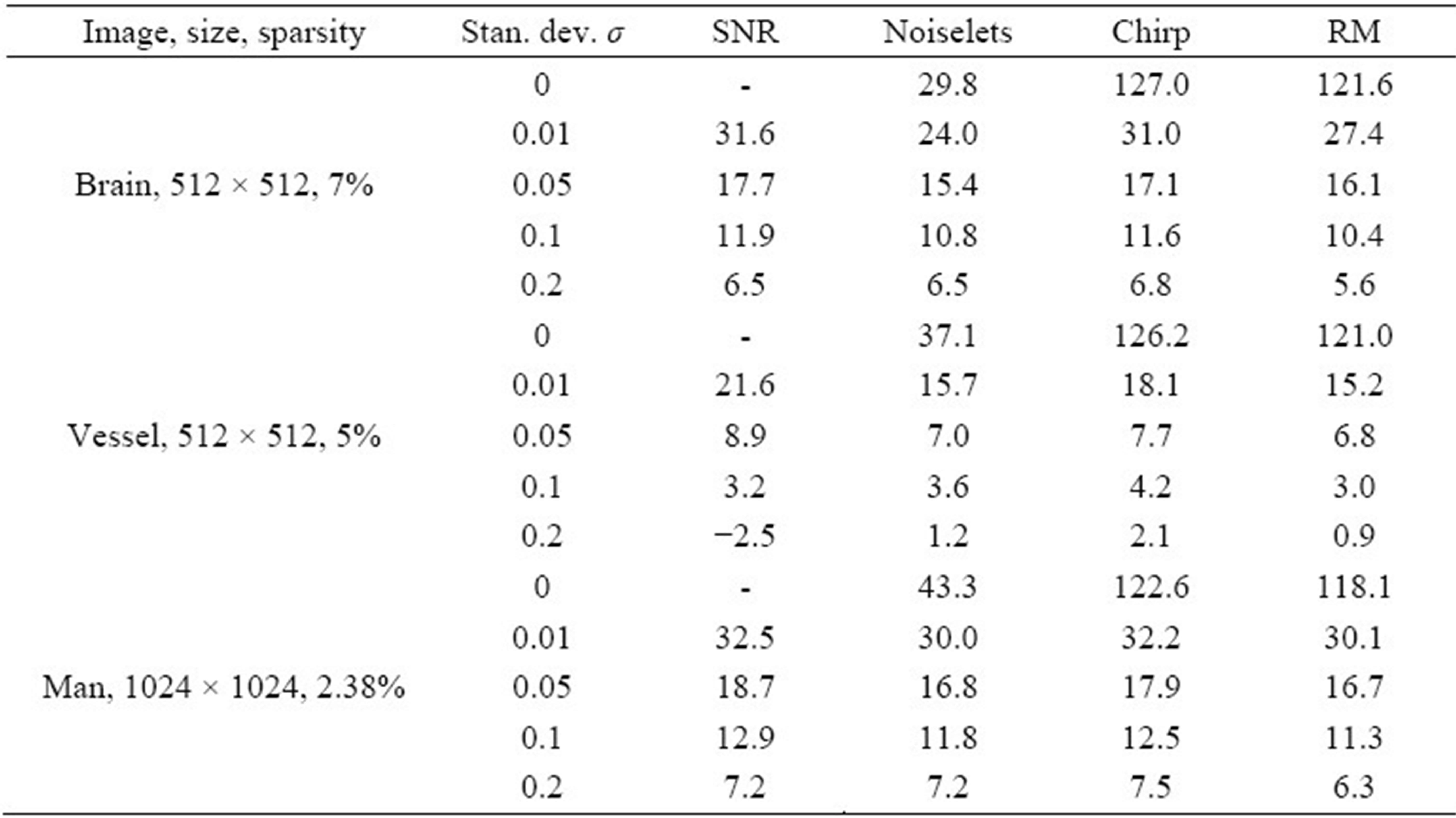
Table 3. In this table, the 2D images are not sparsified. Gaussian noise with zero mean and standard deviation σ is added to all 4 levels of D16 wavelet coefficients decomposition of the non-sparsified image; see (23). The third column shows the SNR in dB of the noisy images compared to the original image. Columns 4-6 show the reconstruction SNR in dB using noiselets, chirp, and Reed-Muller CS algorithms, respectively. The number of measurements taken is 25% of the number of pixels.

lets slightly outperform RM even though the discussion in Section 1 assures that the deterministic compressed sensing matrices comprised of chirps and Reed-Muller sequences have advantage over random matrices. The reason is that the deterministic sensing matrices here satisfy StRIP for sparse signals whose nonzero locations follow a uniform distribution, and the wavelet coefficients do not follow a uniform distribution. Therefore, better performance is not guaranteed anymore. Nevertheless, all results show that the deterministic algorithms are as stable as the reconstruction using noiselets and minimization.

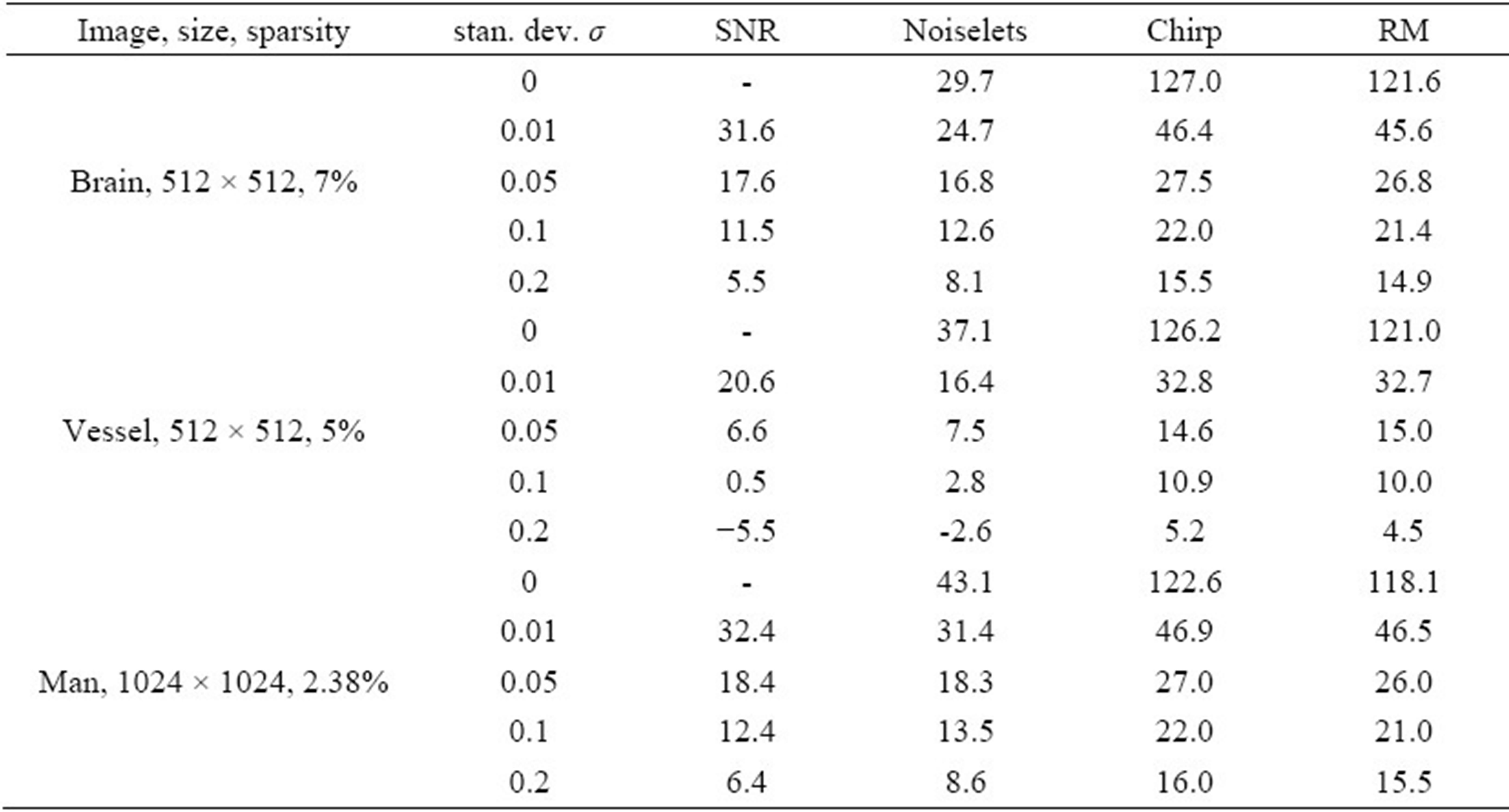
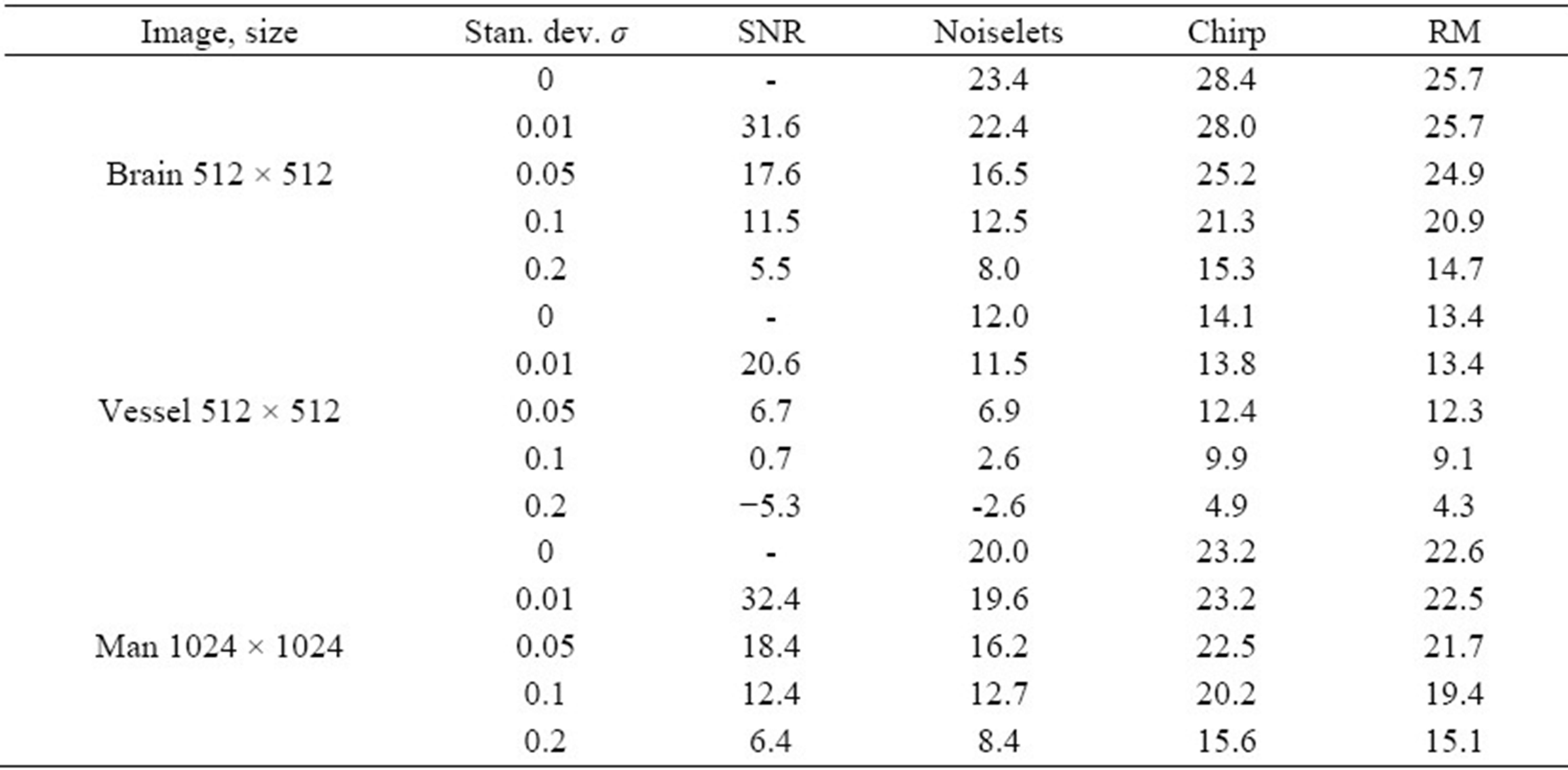
For Tables 5 and 6, the third column gives the SNR of the noisy measurement compared to the clean measurement. The reconstructed SNR is calculated the same way as in Tables 2, 4, and 5, comparing the reconstructed image to the reference image. Therefore, the SNR in the third columns is in a different domain, or differs by the Φ transform. All results show that the reconstruction by chirp or RM performs significantly better than noiselets. Note that in Tables 2-4, where there is no noise, the reconstruction is very accurate, above 100 dB.

Table 4. The 2D images are first sparsified in the Daubechies wavelet D16 domain with 4 levels of decomposition. The pre-determined sparsity for each image is shown in the first column. The Gaussian noise with zero mean and standard deviation σ is added only to the non-zero wavelet coefficients of the sparsified image; see (24). The third column shows the SNR in dB of the images with added noise compared to the noise-free sparsified image. Columns 4-6 show the reconstruction SNR in dB using noiselets, chirp, and Reed-Muller CS algorithms, respectively. The number of the measurements taken is 25% of the number of pixels.

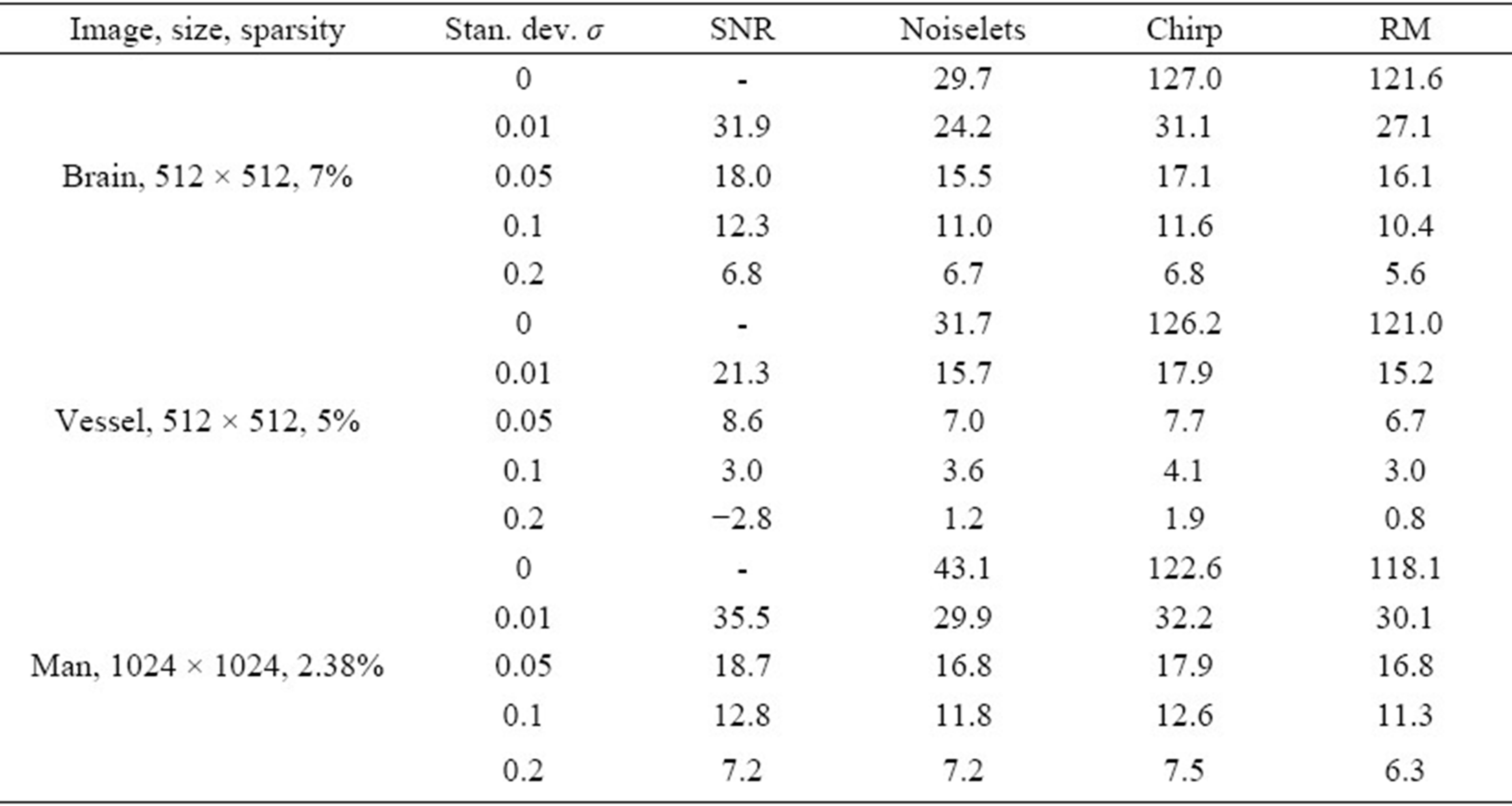
Table 5. The 2D images are first sparsified in the Daubechies wavelet D16 domain with 4 levels of decomposition. The pre-determined sparsity for each image is shown in the first column. Measurements are taken from the D16 domain. The number of measurement taken is 25% of the number of pixels. Gaussian noise with zero mean and standard deviation σ is added to the measurements of the sparsified image; see (25). The third column shows the SNR in dB of the noisy measurements compared to the noise-free measurements. Columns 4-6 show the reconstruction SNR in dB using noiselets, chirp, and Reed-Muller CS algorithms, respectively.

4. Discussions

In this work, we show that the algorithms introduced in [3] are stable even if the signal is not exactly sparse and there is some noise in the measurements or in the signal. We also address several practical concerns about compressed sensing with images.

First of all, the Haar wavelet is commonly used as the sparsifying transform domain. We compare the performance of standard Daubechies DN wavelets and suggest using Daubechies D16 as it performs the best for larger resolutions images, such as 512 × 512 or 1024 × 1024 pixels.

Secondly, we explain the proper selection of the number of levels for wavelet decomposition. As discussed in Section 2, levels 4-7 are optimal for wavelet decomposition, and for optimal computation time we work with level 4.

Table 6. The 2D images are not sparsified in this experiment. Measurements are taken from the D16 domain with 4 levels of decomposition. The number of measurements taken is 25% of the number of pixels. Then, Gaussian noise with zero mean and standard deviation σ is added to the measurements of non-sparsified image; see (26). The third column shows the SNR in dB of the noisy measurements compared to the noise-free measurements. Columns 4-6 show the reconstruction SNR in dB using noiselets, chirp, and Reed-Muller CS algorithms, respectively.

Finally, our experiments show that the algorithms are indeed stable if the signal is compressible and there is noise in either measurements or the signal. Furthermore, our chirp and RM compressed sensing reconstruction algorithms outperform the standard compressed sensing reconstruction using random matrices and minimization. We have also done some analysis on how our efficient reconstruction algorithm can be adapted by using the nesting of the Delsarte-Goethals sets of the ReedMuller codes to deal with very large images. Currently, we are trying to use this to improve the performance of our deterministic compressed sensing algorithms.

5. Acknowledgements

This work is partially supported by NSF-DMS grant #0652833, NSF-DUE #0633033, and ONR-BRC grant #N00014-08-1-1110. The authors are immensely grateful to Douglas Cochran for his invaluable guidance during the course of this work. The authors also wish to express their gratitude to Stephen Howard for many useful discussions.

REFERENCES

Appendix A: SNR values for Figures 2 and 3

Please see Tables A1 and A2.

Table A1. The table below shows reconstruction SNR of chirp compressed sensing with different Daubechies wavelet and 4 levels of decomposition. Specifically, D2 is the Haar wavelet. The 2D images are not sparsified. Each column shows the reconstruction SNR in dB with the indicated DN. The number of measurements taken is 25% of the number of pixels. This table is plotted in Figure 2.

Table A2. The table below shows reconstruction error of chirp compressed sensing with Daubechies D16 wavelet and various levels of decomposition ranging from 3 to 7. The 2D images are not sparsified. Each column shows the reconstruction SNR in dB with the indicated number of levels. The number measurement taken is 25% of the number of pixels. This table is plotted in Figure 3.

NOTES

^*These authors contributed equally to this work.

¹DHT is used for the Reed-Muller sensing matrix while DFT is used in the case of the chirp sensing matrix.

REFERENCES

- K. Ni, P. Mahanti, S. Datta, S. Roudenko and D. Cochran, “Image Reconstruction by Deterministic Compressive Sensing with Chirp Matrices,” Proceedings of SPIE, Vol. 7497, 2009. doi:10.1117/12.832649
- K. Ni, S. Datta, P. Mahanti, S. Roudenko and D. Cochran, “Using Reed-Muller Codes as Deterministic Compressive Sensing Matrices for Image Reconstruction,” Proceedings of the IEEE International Conference on Acoustics, Speech, and Signal Processing, Dallas, 2010, pp. 465-468.
- K. Ni, S. Datta, P. Mahanti, S. Roudenko and D. Cochran, “Efficient Deterministic Compressed Sensing for Images with Chirps and Reed-Muller Sequences,” SIAM Journal in Imaging and Sciences, Vol. 4, No. 3, 2011, pp. 931- 953.
- E. J. Candès, “Compressive Sampling,” Proceedings of the International Congress of Mathematicians, Madrid, 2006, pp. 1433-1452.
- E. J. Candès, J. Romberg and T, Tao, “Robust Uncertainty Principles: Exact Signal Reconstruction from Highly Incomplete Frequency Information,” IEEE Transactions on Information Theory, Vol. 52, No. 2, 2006, pp. 489-509. doi:10.1109/TIT.2005.862083
- D. L. Donoho, “Compressed Sensing,” IEEE Transactions on Information Theory, Vol. 52, No. 4, 2006, pp. 1289-1306. doi:10.1109/TIT.2006.871582
- M. Lustig, D. Donoho and J. M. Pauly, “Sparse MRI: The Application of Compressed Sensing for Rapid MR Imaging,” Magnetic Resonance in Medicine, Vol. 58, No. 6, 2007, pp. 1182-1195. doi:10.1002/mrm.21391
- W. U. Bajwa, J. Haupt, A. M. Sayeed and R. Nowak, “Compressed Channel Sensing: A New Approach to Estimating Sparse Multipath Channels,” Proceedings of IEEE, June 2010, pp. 1058-1076.
- M. Mishali and Y. C. Eldar, “Blind Multiband Signal Reconstruction: Compressed Sensing for Analog Signals,” IEEE Transactions on Signal Processing, Vol. 57, No. 30, 2009, pp. 993-1009.
- T. Lin and F. J. Herrmann, “Compressed Wavefield Extrapolation,” Geophysics, Vol. 72, No. 5, 2007, pp. SM77-SM93. doi:10.1190/1.2750716
- E. J. Candès and T. Tao, “Near Optimal Signal Recovery from Random Projections: Universal Encoding Strategies?” IEEE Transactions on Information Theory, Vol. 52, No. 12, 2006, pp. 5406-5425. doi:10.1109/TIT.2006.885507
- E. J. Candès, J. Romberg and T. Tao, “Stable Signal Recovery from Incomplete and Inaccurate Measurements,” Communications on Pure and Applied Mathematics, Vol. 59, No. 8, 2006, pp. 1207-1223. doi:10.1002/cpa.20124
- E. J. Candès and J. K. Romberg, “Signal Recovery from Random Projections,” Proceedings of SPIE, Vol. 5674, 2005, pp. 76-86.
- R. DeVore, “Deterministic Constructions of Compressed Sensing Matrices,” Journal of Complexity, Vol. 23, No. 4-6, 2007, pp. 918-925. doi:10.1016/j.jco.2007.04.002
- L. Applebaum, S. D. Howard, S. Searle and R. Calderbank, “Chirp Sensing Codes: Deterministic Compressed Sensing Measurements for Fast Recovery,” Applied and Computational Harmonic Analysis, Vol. 26, No. 2, 2009, pp. 283-290. doi:10.1016/j.acha.2008.08.002
- S. D. Howard, A. R. Calderbank and S. J. Searle, “A Fast Reconstruction Algorithm for Deterministic Compressive Sensing using Second Order Reed-Muller Codes,” Proceedings of the Conference on Information Sciences and Systems, Princeton, 2008, pp. 11-15.
- R. Calderbank, S. Howard and S. Jafarpour, “Construction of a Large Class of Deterministic Matrices that Satisfy a Statistical Isometry Property,” IEEE Journal on Selected Topics in Signal Processing, Vol. 29, No. 4, 2009, pp. 358-374.
- P. Indyk, “Near-Optimal Sparse Recovery in the L1 Norm,” 49th Annual IEEE Symposium on Foundations of Computer Science, Philadelphia, 25-28 October 2008, pp. 199-207.
- E. J. Candès and J. Romberg, “Sparsity and Incoherence in Compressive Sampling,” Inverse Problems, Vol. 23, No. 3, 2007, pp. 969-985. doi:10.1088/0266-5611/23/3/008
- D. Baron, M. F. Duarte, S. Sarvotham, M. B. Wakin and R. G. Baraniuk, “An Information-Theoretic Approach to Distribute Compressed Sensing,” Proceedings of the 43rd Allerton Conference on Cozmmunications, Control, and Computing, Allerton, September 2005.
- W. O. Alltop, “Complex Sequences with Low Periodic Correlations,” IEEE Transactions on Information Theory, Vol. 26, No. 3, 1980, pp. 350-354. doi:10.1109/TIT.1980.1056185
- K. J. Horadam, “Hadamard Matrices and Their Applications,” Princeton University Press, Princeton, 2007.
- A. Roger Hammons Jr., P. Vijay Kumar, A. R. Calderbank, N. J. A. Sloane and P. Solé, “The
-Linearity of Kerdock, Preparata, Goethals, and Related Codes,” IEEE Transactions on Information Theory, Vol. 40, No. 2, 1994, pp. 301-319. doi:10.1109/18.312154
- R. Calderbank, “Personal Communication,” 2009.
- A. M. Kerdock, “A Class of Low Rate Nonlinear Binary Codes,” Information and Control, Vol. 20, No. 2, 1972, pp. 182-187. doi:10.1016/S0019-9958(72)90376-2
- C. C. Paige and M. A. Saunders, “LSQR: An Algorithm for Sparse Linear Equations and Sparse Least Squares,” ACM Transactions on Mathematical Software, Vol. 8, No. 1, 1982, pp. 43-71.
- T. Faktor, Y. C. Eldar and M. Elad, “Exploiting Statistical Dependencies in Sparse Representations for Signal Recovery,” IEEE Transactions on Signal Processing, Vol. 60, No. 5, 2012, pp. 2286-2303.
- C. La and M. N. Do, “Tree-Based Orthogonal Matching Pursuit Algorithm for Signal Reconstruction,” 2006 IEEE International Conference on Image Processing, Atlanta, 8-11 October 2006, pp. 1277-1280.
- Y. C. Eldar and M. Mishali, “Robust Recovery of Signals from a Structured Union of Subspaces,” IEEE Transactions on Information Theory, Vol. 55, No. 11, 2009, pp. 5302-5316. doi:10.1109/TIT.2009.2030471
- Y. C. Eldar, P. Kuppinger and H. Bölcskei, “Compressed Sensing of Block-Sparse Signals: Uncertainty Relations and Efficient Recovery,” 2010. arXiv:0906.3173
- J. Romberg, “Imaging via Compressive Sampling,” IEEE Signal Processing Magazine, Vol. 25, No. 2, 2008, pp. 14-20.