Applied Mathematics
Vol. 3 No. 2 (2012) , Article ID: 17384 , 8 pages DOI:10.4236/am.2012.32020
Wavelet Optimized Adaptive Mesh for MHD Flow Problems
1Jaypee Institute of Information Technology, Noida, India
2Department of Mathematics, Vishveshwarya Institute of Engineering & Technology, Nagar, India
Email: *anujbhardwaj8@gmail.com
Received December 12, 2011; revised January 17, 2012; accepted January 25, 2012
Keywords: MHD flow; Interpolating Wavelet; Adaptive Mesh
ABSTRACT
There are many problems in science and engineering where the solution shows a boundary layer character. Near the boundary the gradient is large in contrast with the smooth behaviour in the central core. A uniform grid is, therefore, not suitable for a numerical solution. MHD flow problems belong to this category where a velocity and induced magnetic field profiles get flattened in a transverse flow. In the present paper an optimized grid has been generated using interpolating wavelets. The results are compared with those obtained using uniform grid, the finite element method and also from the analytical solution.
1. Introduction
Study of MHD flows is important due to a number of applications in science and engineering. Since blood is electrically conducting several papers have appeared in literature on the blood flow control and measurements [1,2]. Other applications are in MHD flowmetry, MHD power generation. The study of generation and maintenance of magnetic field in steller bodies like the Sun and the Earth is owing to the constant motion of conducting material inside these bodies [3]. Some of these are cited in the references [4-8]. These are the problems where we study the effect of the transverse magnetic field on the flow of electrically conducting fluid. There is, therefore, a complex interaction of the equations of electrodynamics and fluid mechanics. The magnetic lines of force act like stretched rubber bands which try to reduce the flow rate. Therefore, a component of magnetic field is generated in the direction of the fluid flow. This is called the induced magnetic field. The main aim of all the MHD flow studies is to compute the modified flow pattern and the induced magnetic field. In our earlier paper [9] we solved an MHD flow problem which involved solving a singular integral equation. Haar wavelets with special integration formulae over boxes with singularities were used.
In the present paper we solve a different problem using wavelet optimized adaptive mesh. This method has been developed very recently and has become a very popular numerical tool to solve the boundary value problems where the rates of variation of the dependent variable significantly vary in the domain of interest. Of particular interest are the problems where there is a boundary layer in which the gradients are very steep as compared with the core where the variations are negligible. While applying finite difference or finite element method one has, therefore, to take a variable mesh—a finer one in the boundary layer and a coarser one in the core region. The main question is how to choose the size. There are several methods to choose a variable mesh a priori. One method frequently used is the “geometric mesh” in which the mesh size decreases in the geometric progression. We can control it by taking common ratio as a parameter. The other well known way is to use the chebyshev mesh. None of these is of adaptive nature since we choose it beforehand. In the wavelet method the mesh size is automatically adjusted keeping in view the rates of variation. For this we compute and test the magnitudes of the wavelet coefficients in the wavelet approximation. We stop reducing the mesh size when these coefficients become smaller than a prescribed quantity. Once the mesh size is decided we discretize the governing equations and solve the resulting system of algebraic equations. Some important references where this technique has been successfully used are [10-16].
2. Basic Equations
The basic equations of MHD are very well-known [4,8, 17,18]. We do not go into their derivation and the necessary physics involved in it. Figure 1 shows the section of the straight rectangular pipe of uniform cross-section and non-conducting walls. The flow of the electrically conducting fluid is axial i.e. along z-axis taken out of paper. The applied transverse magnetic field is along x-axis. The induced magnetic field is created along the flow direction. The final equations is a coupled system in the induced magnetic field  and the axial velocity
  in non-dimensional form
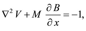 (1)
(1)
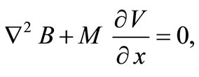 (2)
(2)
in the flow region bounded by  and
and  Here
Here  and
and  are the velocity and the induced magnetic field along z-axis at the point
 . The non-slip condition and non-conducting nature of the walls lead to the following boundary conditions.
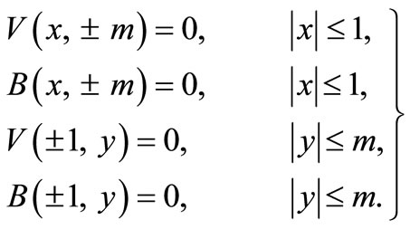 (3)
(3)
The non-dimensional parameter  is called the Hartmann number. It is a measure of the intensity of the applied magnetic field. The analytical solution of (1) and (2) with boundary conditions (3) is known in [4-6]. It can be expressed as [7].
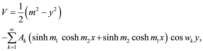 (4)
(4)
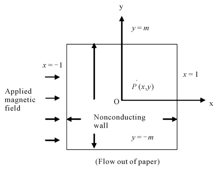
Figure 1. Section of the channel.
 (5)
(5)
where
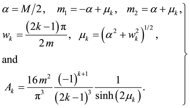 (6)
(6)
From (4) and (5)  and
and  can be computed for a given
  at any point
  of the cross-section. But there are difficulties when
  is large. The boundary layer character of the problem can be easily recognized from (1) and (2) when
  is large. One can separately solve in the boundary layer and core region and match the two solutions at the interface. Another approach is to use finite difference or finite element methods (FEM) with finer mesh near the walls and a coarser mesh in the core region. Singh and Lal in [7] have used the FEM for various Hartmann numbers.
3. Present Method—The Wavelet Optimized Adaptive Mesh (WOAM)
Wavelets can be used to obtain the optimum size of the mesh in the flow region for different Hartmann numbers and specified precision. As  increases the mesh becomes finer and finer near the boundary. In the present problem the boundary layers are more pronounced at
  as compared to
 . As a result of this different mesh sizes are obtained along
  and y-directions. This is further compounded by the fact that there are two dependent variables
  and
and  and at a time we can optimize with respect to one of them only. Fortunately, both the variables depict similar behaviour as
  increases. So we have optimized with respect to
  only. To get an idea about the boundary layers, we have plotted velocity profiles along x-axis (Figure 2) for different Hartmann numbers. The case
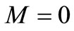 , corresponds to the hydrodynamic case. It can be seen that as
  increases the core profile becomes more and more flat in the core region. This is further confirmed by Figure 3 which shows contours of
 .
.
To get the optimized mesh we have constructed interpolating wavelets of [10,11] in both the x and y-directions for a given Hartmann number. After having generated the mesh the derivatives at the non-uniform mesh are approximated as described by Jameson [12]. We obtain the interpolating wavelets on the dyadic grid  along x-axis defined by
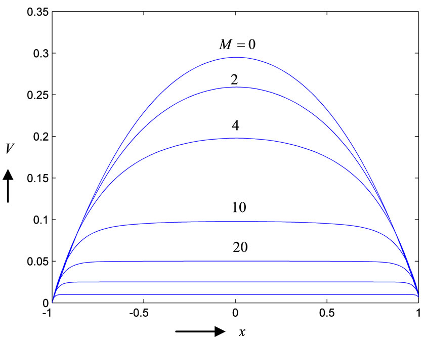
Figure 2. Velocity profiles along x-axis for M = 0, 2, 4, 10, 20, 40 and 100 (M = 0 is at the top and M = 100 at the bottom).
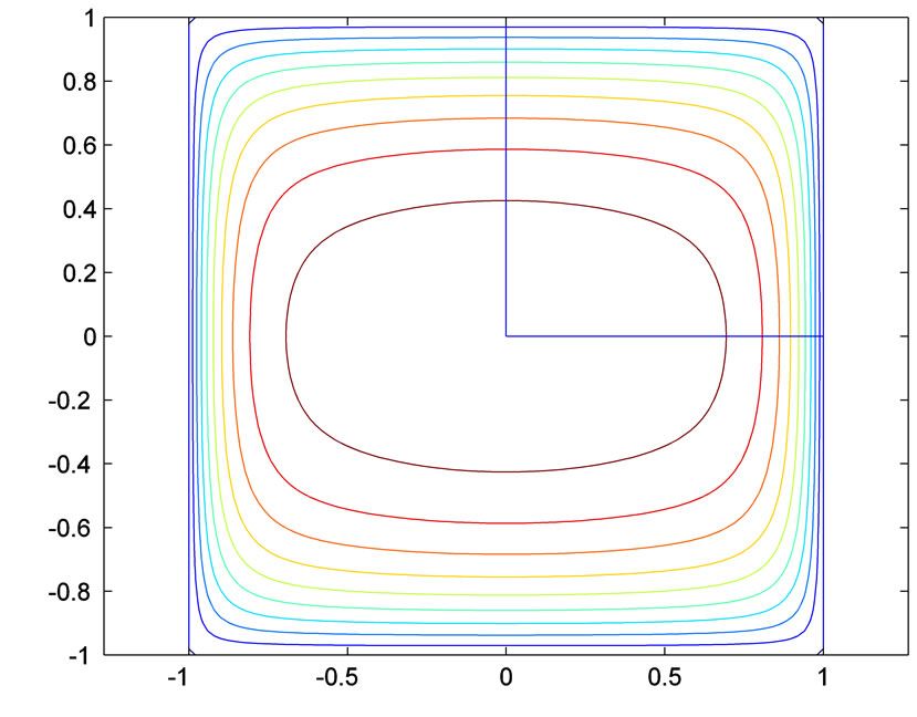
Figure 3. Contour lines for M = 10.
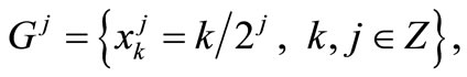 (7)
(7)
where  is the set of integers with
  as the level of resolution. The algorithm proceeds from the level
  to level
  by interpolating at the additional points of
  using the data sequence
  defined at
 . For this purpose the nearest
  points are used. This gives
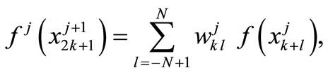 (8)
(8)
where  are weights. Note that the weights do not change with
  for evenly spaced grid. However, we can easily extend them to a non-uniform grid. Generalization of the above procedure to intervals is also straightforward. A suitable modification is to be made near the ends of the interval. The interpolating function
 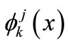 can be defined by setting
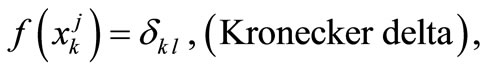 (9)
(9)
and applying the algorithm upto a high level  of resolution. This will result in the scaling function sampled at the locations
 . Using linear superposition we have
 (10)
(10)
with
 (11)
(11)
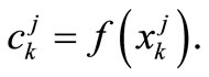
Figures 4 and 5 depict the graphs of scaling functions  for
for  and 3 respectively.
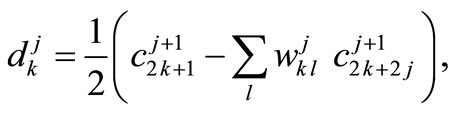
Proceeding as in [13,14], we define the wavelet coefficients
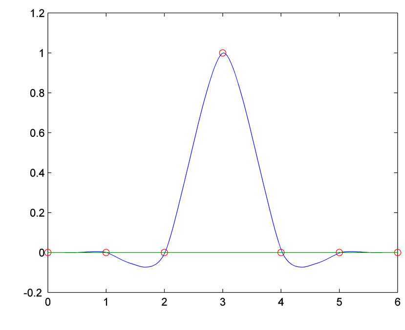
Figure 4. Scaling function  for N = 2.
Figure 5. Scaling function  for N = 3.
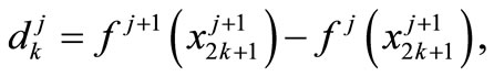 (12)
(12)
and set
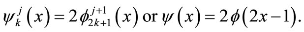 (13)
(13)
This gives the detail function
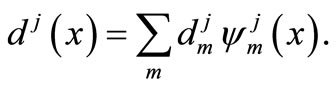 (14)
(14)
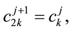
Then
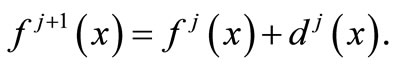 (15)
(15)
The forward and inverse wavelet transform are, therefore, defined by
 (16)
(16)
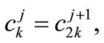 (17)
(17)
 (18)
(18)
and
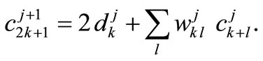 (19)
(19)
To generate the adaptive mesh we, therefore, proceed as follows:
1) Obtain the solution at the coarser mesh to get the initial profile.
2) Apply wavelet transform to get the wavelet coefficients  These are expected to be large where the gradient is high i.e. boundary layers and small where solution is smooth, i.e. core region.
3) Remove the mesh points where , where
  is the specified tolerance. Retain the additional points where
4) Continue modifying the mesh till (3) is satisfied everywhere.
The above procedure will result in a finer mesh in the boundary layers but coarser in the core region.
4. Numerical Results, Convergence and Discussion
We have applied the above procedure for the pipe of square cross-section  for different Hartmann numbers. The initial mesh size is taken as 0.1 and
  is taken as
  for all Hartmann numbers. The value of
  has been chosen to be 2. The final mesh will obviously depend on
  and also
 . For example, for
 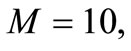 we obtained the mesh as shown in Figure 6. In the region
  the mesh size is 0.1. It falls to 0.05 and remains so upto
  After that it gets reduced to 0.025 and so on. As
  increases the rate of change of
  increases and, therefore, the mesh size has to be re-
Figure 6. Adaptive mesh for M = 10, N = 2.
duced. Upto  the condition
  is satisfied if mesh size is 0.1 (or less). For having optimum size we take it as 0.1. When
  is further increased the condition
  is not satisfied so size is reduced by a factor of half. With this size the condition remains satisfied upto
  After that it is further reduced and so on.
Fortunately, the following symmetric considerations permit the equations to be solved in the positive quadrant only
 (20)
(20)
 (21)
(21)
The solution is found at the internal nodes
where  depend on the Hartmann number.
Tables 1 and 2 give the velocity and induced magnetic field for  and
and  at the selected common points of the mesh. The exact values as computed from the analytical solution are also given for comparison. Figures 7 and 8 give the three dimensional profiles of
  and
and  over the entire section for
  Table 3 gives the values of
  at the centre of the section. Values as obtained using the uniform mesh with the same number of nodes are also given as
  (Velocity for uniform mesh). Comparison is also made with the values obtained using FEM. Comparison at points other than centre was not possible because there are no other common points. It is clear from the tables that the results from the adaptive mesh are consistently better than those obtained using uniform mesh and the FEM.
The pointwise convergence of results with varying  for different Hartmann numbers is clear from the Table 4 which gives errors in the computed values at the centre
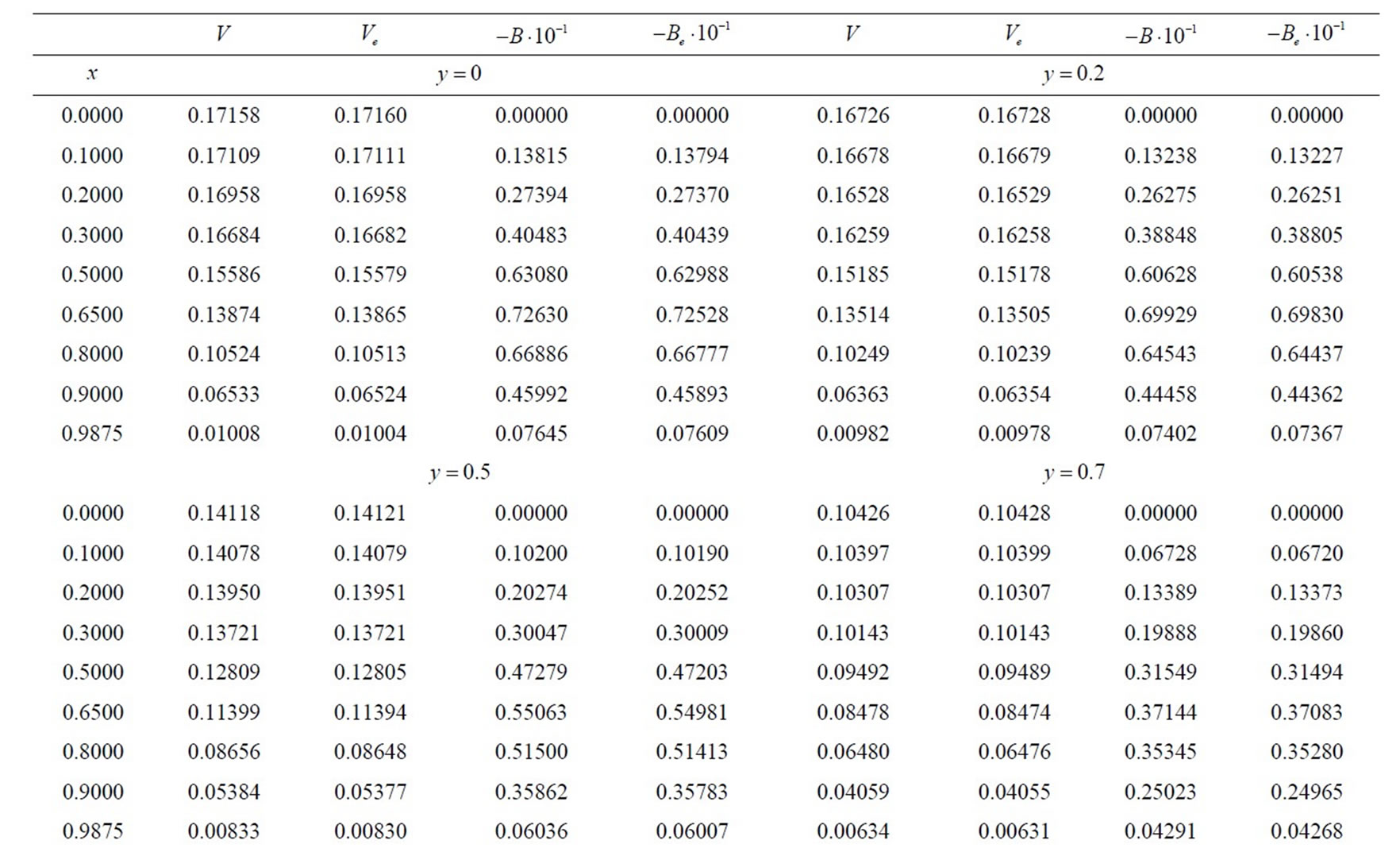
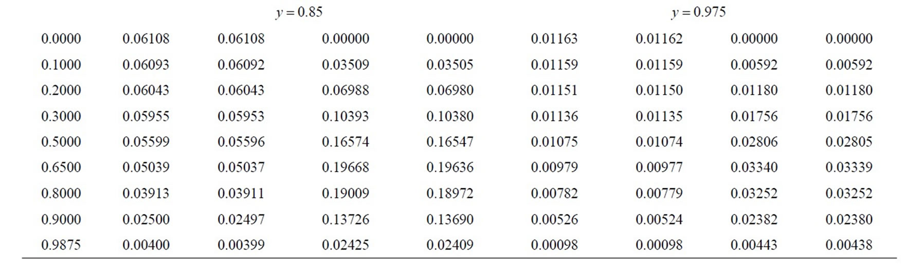
Table 1. Velocity and induced magnetic field at selected points for M = 5.
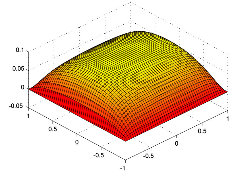
Figure 7. Velocity profile for M = 20.
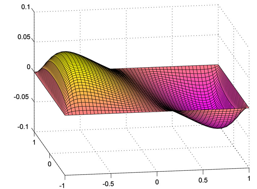
Figure 8. Magnetic field profile for M = 20.
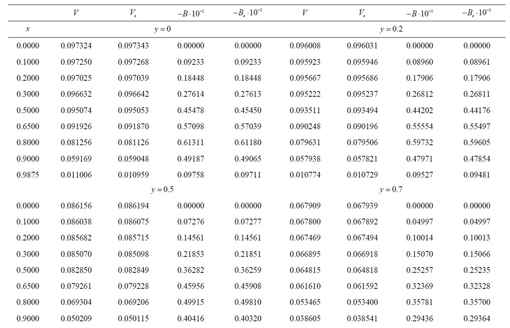
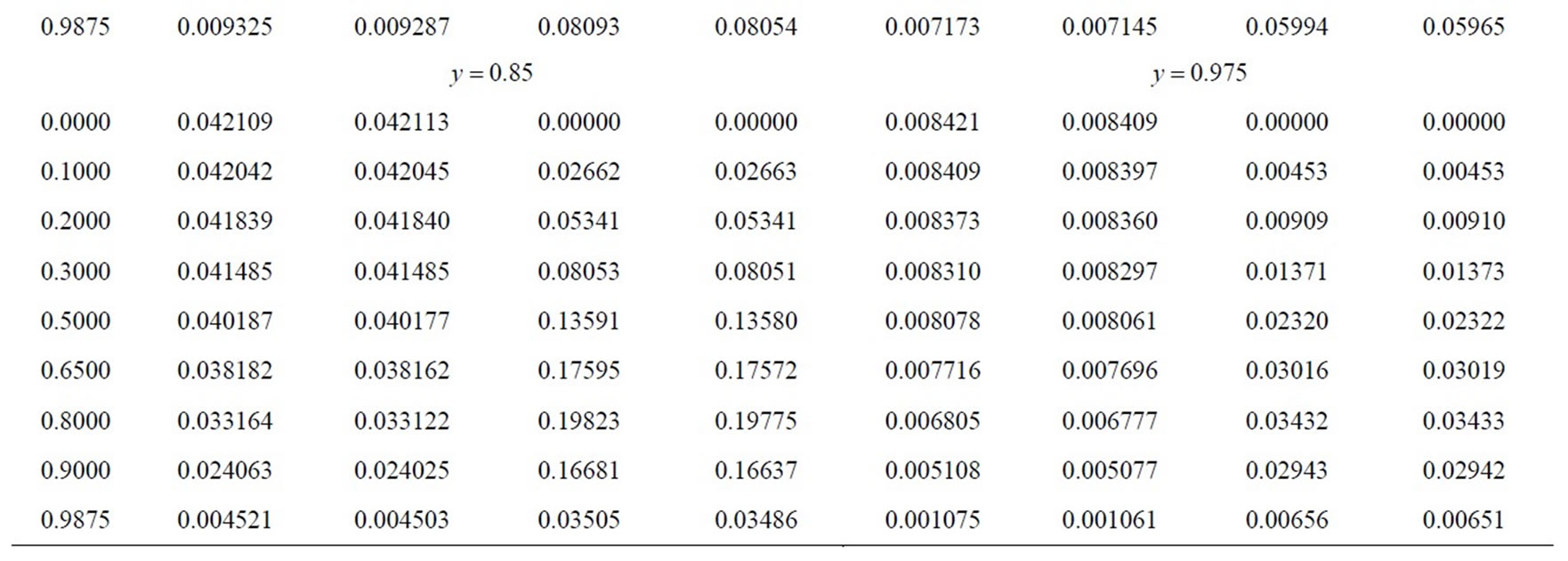
Table 2. Velocity and induced magnetic field at selected points for M = 10.
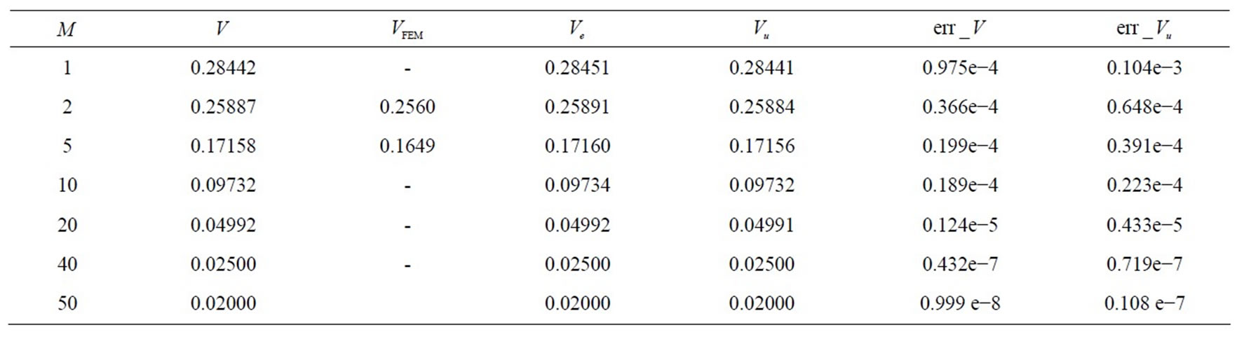
Table 3. Comparison of velocity at the centre by different methods.
of the channel. This point has been chosen because it is common to all the meshes. It is seen that as  is increased the error also increases. Interestingly, errors are lower for large Hartmann numbers clearly demonstrating the suitability of the present method to the situations where variations in the central core are far less than in the boundary region.
The overall convergence in the entire section is clear from Table 5 which gives the mean absolute error (MAE) and root mean square error (RMSE) for various Hartmann numbers and . It is clear that as
  is reduced the errors both MAE and RMSE get reduced. Again the results are more encouraging for large
  From these observations we can conclude that the present method is ideally suited to problems depicting the boundary layer character.
5. Observation, Conclusion and Future Scope
As pointed out in the introduction, the basic aim of the present study was to solve the problem numerically using wavelet optimized adaptive mesh. This method is of recent origin and has been successively applied in many other applications. As explained above the method is suitable to the MHD flow problems also due to their boundary layer character. The uniform mesh is not appropriate near the boundaries and to use a fine mesh in the entire domain leads to excessive computation time. The adaptive mesh using wavelets gives good accuracy even with moderate size of the mesh. A mesh where size is pre-decided such as the “geometric mesh” or “chebyshev mesh” also do not serve the complete purpose because the rate of variation of  may not be consistent with the rate of variation of the mesh size. The adaptive mesh on the other hand adapts its size according to the rate at which
  varies. For a given
  it is also optimum since we reduce the size by a factor of half only when the specified tolerance is not satisfied.
In future we intend to extend the method to other geometries such as circular and elliptic. All the problems which have come to our notice in literature where wavelet adaptive mesh has been applied are one dimensional. The present paper extends it to two dimensions. The rates of variations near the boundary have been very fast along x-axis but comparatively not that fast along y-axis. Accordingly, the adaptive meshes are different along both directions. When we take a circular geometry, many unexpected problems arise. One of them is the choice of grid-rectangular or polar. Each has its advantages and disadvantages. Near the boundaries the finite difference approximations become very poor. We are trying to overcome these problems. We are also trying to examine whether the method in the present form is suitable for complex geometries. A suitable combination of it with FEM and the Boundary Integral Equation Methods (BIEM) may be a better alternative. We are currently working in this direction.
6. Acknowledgements
The authors are thankful to Dr. Mani Mehra (IIT, Delhi)
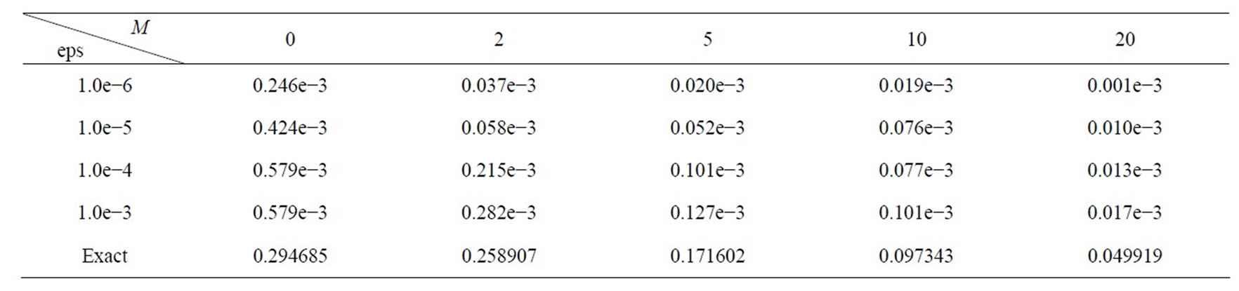
Table 4. Convergence of results for velocity V at the centre of section (n = 2 starting mesh size h = 0.1).
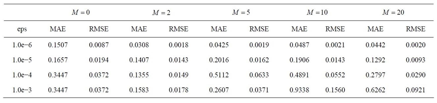
Table 5. Mean Absolute Error (MAE) and Root Mean Square Error (RMSE) in computed values of V over the section (multiply by 10−3).
and Dr. Vivek Kumar (JIIT) for helpful discussions.
REFERENCES
- A. Kolin, “An Electromagnetic Flowmeter—The Principle and Its Applications to Blood Flow Measurement,” Proceedings of the Society for Experimental Biology and Medicine, Vol. 35, 1936, pp. 53-56.
- A. Kolin, “Electromagnetic Blood Flow Meters,” Science, Vol. 130, No. 3382, 1959, pp. 1088-1097. doi:10.1126/science.130.3382.1088
- J. A. Jacobs, Ed., “Geomagnetism I and II,” Academic Press, Cambridge, 1987.
- J. A. Shercliff, “Steady Motion of Conducting Fluids in Pipes under Transverse Magnetic Fields,” Mathematical Proceedings of the Cambridge Philosophical Society, Vol. 49, No. 1, 1953, pp. 136-144. doi:10.1017/S0305004100028139
- C. C. Changa and T. S. Lundgren, “Duct Flow in Magnetohydrodynamics,” Zeitschrift für Angewandte Mathematik und Physik (ZAMP), Vol. 12, No. 2, 1961, pp. 100-114.
- J. C. R. Hunt, “Magnetohydrodynamic Flow in Rectangular Duct,” Journal of Fluid Mechanics, Vol. 21, No. 4, 1965, pp. 577-590. doi:10.1017/S0022112065000344
- B. Singh and J. Lal, “Finite Element Method in Magnetohydrodynamic Channel Flow Problems,” International Journal for Numerical Methods in Engineering, Vol. 18, No. 7, 1982, pp. 1104-1111. doi:10.1002/nme.1620180714
- B. Singh and J. Lal, “Finite Element Method for Unsteady MHD Flow through Pipes with Arbitrary Wall Conducting,” International Journal for Numerical Methods in Fluids, Vol. 4, No. 3, 1984, pp. 291-302. doi:10.1002/fld.1650040307
- B. Singh, A. Bhardwaj and R. Ali, “A Wavelet Method for Solving Singular Integral Equation of MHD,” Applied Mathematics & Computation, Vol. 214, No. 1, 2009, pp. 271-279. doi:10.1016/j.amc.2009.03.075
- D. L. Donoho, “Interpolating Wavelet Transform,” Technical Report, Stanford University, Palo Alto, 1992.
- A. Harten, “Adaptive Multiresolution Schemes for Shock Computations,” Journal of Computational Physics, Vol. 115, No. 2, 1994, pp. 319-338. doi:10.1006/jcph.1994.1199
- L. Jameson, “A Wavelet Optimized Very High Order Adaptive Grid and Numerical Method,” SIAM Journal on Scientific Computing, Vol. 19, No. 6, 1998, pp. 1980- 2013. doi:10.1137/S1064827596301534
- O. V. Vasilyev and C. Bowman, “Second Generation Wavelet Collocation Method for Solution of Partial Differential Equations,” Journal of Computational Physics, Vol. 165, No. 2, 2000, pp. 660-693. doi:10.1006/jcph.2000.6638
- V. Kumar and M. Mehra, “Wavelet Optimized Finite Difference Method Using Interpolating Wavelets for Self Adjoint Singularly Perturbed Problems,” Journal of Computational and Applied Mathematics, Vol. 230, No. 2, 2009, pp. 803-812.
- I. Fatkulin and J. S. Hesthaven, “Adaptive High-Order Finite Difference Method for Nonlinear Wave Problems,” Journal of Scientific Computing, Vol. 16, No. 1, 2001, pp. 44-67. doi:10.1023/A:1011198413865
- Z.-L. Pei, L.-Y. Fu, G.-X. Yu and L.-X. Zhang, “A Wavelet-Optimized Adaptive Grid Method for Finite-Difference Simulation of Wave Propagation,” Bulletin of the Seismological Society of America, Vol. 99, No. 1, 2009, pp. 302-313. doi:10.1785/0120080002
- J. Hartmann, “Hg-Dynamics I—Theory of Laminar Flow of an Electrically Conducting Liquid in a Homogeneous Magnetic Field,” Kongelige Danske Videnskabernes Selskab. Mathematisk-fysiske Meddelelser, Copenhagen, Vol. 15, No. 6, 1937.
- R. R. Gold, “Magnetohydrodynamic Pipe Flow—Part I,” Journal of Fluid Mechanics, Vol. 13, No. 4, pp. 505-512. doi:10.1017/S0022112062000889
NOTES
*Corresponding author.