ABSTRACT

The paper examines the case of splitting a defaulted mortgage loan on a commercial property into an A note that earns interest and a B note that earns a return only if the value of the property increases. The B note is known as a “hope note.” The paper shows that the current methods for structuring such a deal often produce a B note that is worthless. A state-preference model is employed.

1. Introduction: A Hope Note Example

A Wall Street Journal article by Yoon [1] reports an example of a “hope note.” Gotham Realty Holdings defaulted on a $90 million mortgage taken in 2007 on a commercial property in Manhattan. The loan servicer, Bowery Savings Bank, sought to avoid foreclosure by splitting the mortgage into two parts; the A note is $65 million that will continue to pay interest until maturity in 2017, and the B note (the hope note) is $25 million that pays no interest but is to receive a return when the building is sold. The A note reportedly represented more than 100% of the appraised value at the time the note was issued in 2011, so that holders of the A note had a claim that was greater than the estimated value of the property when the notes were created.  Holders of the A note, in addition to interest payments, receive repayment of principle and some of the appreciation in value. Yoon [1] does not specify the appraised value. The B note was to earn a return when the building is sold if there is appreciation in value sufficient to pay the amounts due the A note (and any new investments made in the building). SL Green Realty Corp. took control of the property after Gotham Real Holdings defaulted and refinanced the loan in 2012. The proceeds from the sale of the A note fell short of $65 million by just $103,000, and the B note was written off as worthless. The loss on the B note was $18.1 million, the size of the note when it was created. The occupancy rate in the building fell from 98% in 2007 to 70% in 2012, and the debt service ratio (net operating income divided by debt service) never reached the projected level of 1.26. The B note is an example of an attempt to introduce a form of equity participation to work out a default.

The A note is defined as the senior portion of the original debt that receives interest payments until the property is sold, has its principle repaid upon the sale of the property, and also receives a portion of any capital appreciation—based on the selling price minus the appraised value of the property at the time the A and B notes are created. The B note receives the remaining portion of any additional appreciation in value, but receives no periodic interest payments. Yoon [1] also reports that a study by Credit Suisse of 15 modifications that included B notes (hope notes) found that seven of the B notes were 100% losses, five had no loss, and three had losses less than 100%. Why do hope notes often turn out to have been hopeless?

This paper employs a basic state-preference model to value the A and B notes (and their sum) to show that the B note has value only if the expected appreciation in value exceeds the amount of appreciation that is due to the holders of the A note. If the amount due on the A note is set too high, the B note is worthless. The value of the sum of the A and B notes does not depend upon the split of the appreciation in value between the two notes.

2. A State-Preference Model

The state-preference approach was introduced by Arrow [2] and adapted by Stiglitz [3], Sargent [4], and McDonald [5] to illustrate the Modigliani-Miller [6] Proposition I.This section outlines the state-preference approach and applies it to an individual firm, as in McDonald [5].

Arrrow [2] assumes that there is only one date in the “future,” and that there are N possible future states of the world. The index of future states of the world is. There are C commodities and each individual has a quasi-concave utility function U; utility is a function of the future state of the world and the amount of each commodity consumed at that time. Consumption by individual i in state of the world θ of commodity c is denoted x_iθc. The utility function for individual i is

(1)

This formulation is analogous to a utility function under certainty except that the number of variables is increased from C to NC. Each individual has subjective probabilities regarding the future states of the world. Arrow [2, p. 92] proves the following: “… any optimal allocation of risk-bearing can be realized by a system of perfectly competitive markets in claims on commodities.” Prices are established for a unit claim on each commodity if each state of the world occurs, and the individual responds to those prices. There exists a set of such prices and money incomes for the consumers that are consistent with any optimal allocation of risk bearing. As Arrow [2] points out, the theorem is a rather trivial extension of the usual welfare economics theorem. Arrow [2] goes on to prove that the same optimality result can be achieved with a set of perfectly competitive markets for securities payable in money rather than specific individual commodities. When a state of the world occurs money is paid out, and the allocation of commodities proceeds though the market without additional risk bearing.

The model adopted by Stiglitz [3], Sargent [4], and McDonald [5] makes the simplifying assumption that utility depends upon the future state of the world and the amount of money M in his/her possession at that time:

(2)

The individual has a set of subjective probabilities over the states of the world that sum to 1.0. Individuals are assumed to maximize expected utility V:

(3)

The individual is assumed to have an endowment of M⁰ at the present that is invested to provide for future consumption.

Consider a competitive economy in which there are N markets for contingent (Arrow-Debreu) securities, where each one promises to pay one dollar if the corresponding state of the world θ occurs. The price of a security, , is the price of the claim on one dollar should state θ occur. The units of are dollars in the current period per dollar in state θ in the future. The price of a certain dollar in the future is, which is the reciprocal of one plus the risk-free interest rate. Perfect markets for contingent securities in all states of the world mean that it is possible to insure against any risk.

The individual faces the Arrow-Debreu budget constraint that states:

(4)

Since it is assumed that a complete set of markets for contingent securities exists, and if there is general agreement about the probabilities for the future states of the world, the prices for the contingent securities are actuarially fair; i.e.,

(5)

where and are the prices of the contingent securities for states of the world i and j, and and are the probabilities of states of the world i and j. As Nicholson [7, pp. 228,229] points out in a textbook presentation of the model, fair markets for these contingent claims securities are analogous to insurance markets or odds for horse races that reflect true probabilities. Maximization of utility subject to the budget constraint produces the condition for the marginal rate of substitution between money in any two states of the world:

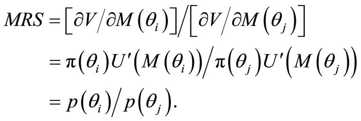(6)

Since the market for contingent securities is actuarially fair, this first-order condition reduces to

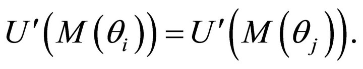(7)

Assuming that the utility function is the same regardless of the future state of the world, Equation (7) means that. In short, the individual acts to insure that the level of money in the future is the same amount regardless of the future state of the world. The individual invests M⁰ in Arrow-Debreu securities based on equity in firms and bonds to generate this amount of money in the future, and earns the risk-free rate of return. It is important for understanding the model to recall that individuals invest in a complete set of Arrow-Debreu securities based on both stocks and bonds. Firms and issuers of bonds are intermediaries that provide the investment vehicles upon which Arrow-Debreu securities are based.

Now consider firms that produce output that individuals purchase in the future. We assume an absence of taxes. A firm produces a return net of current labor and materials costs that depends upon the state of the world;. The firm issues bonds in the amount of B dollars, and promises now to pay to its bond holders at the future date, provided that the firm is not bankrupt at that time; i.e.,. The rate at which the firm borrows is r, and the rate that it pays its lenders is. The firms goes bankrupt if, so the realized returns to bonds depend upon the state of the world as follows.

Return to bond

or

(8)

The model includes possible bankruptcy so that there is a need for financial intermediation. The amount cB is the cost of providing the financial intermediation services in which it was determined that the firm was in fact eligible to borrow amount B. It is assumed that this cost must be paid in full unless; in this case the lender suffers a loss. The case in which the future value of the firm is less than the outstanding balance of the loan occurs if (in real estate known as being under water).

The value of the firm’s bonds is equal to the sum of the values of the contingent securities on which the bond consists implicitly. States of the world in which the firm does not go bankrupt are indexed as, and states of the world in which the firm goes bankrupt are indexed as. The value of the firm’s bonds to the lenders is:

(9)

The price vector is set by the market so that the lender earns the risk-free rate of return. The value of the firm’s equity is:

(10)

Therefore, the value of the firm V is:

(11)

so        

The risk-free interest rate is denoted r_f. The value of the firm decreases with both the amount borrowed and the cost of financial intermediation. If the borrowing and lending rates are equal, then and the value of the firm does not depend upon borrowing. This is, of course, Modigliani-Miller Proposition I. Note that it is possible to insure against any risk in this model.

3. Equity Participation

A hope note is a special form of equity participation in which two notes are created that share in any appreciation in value of the property. It is helpful to examine the standard case of equity participation first. See McDonald [8] for a more thorough examination of equity participation loans. Equity participation usually involves the lender accepting a reduction in the interest rate on the loan for a share of the return to equity. Assume that the share of the return to equity for the lender is s and the new (lower) interest rate on the loan is. The value of that equity share E_L is

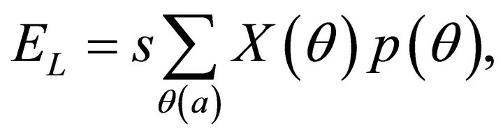(12)

and the value of the firm’s equity is now

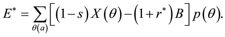(13)

The value of the firm’s bond to the lender is

(14)

Therefore the value of the firm is now the same as in Equation (11);

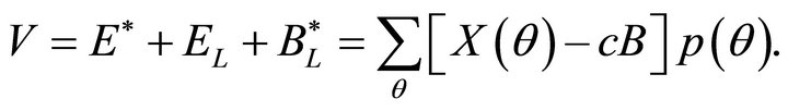(15)

The value of the firm is unchanged, and the terms of the equity participation do not matter (i.e., the choices of s and). Indeed, the interest rate on the loan could be greater than r and still the value of the firm is unchanged.

The conversion of a portion of debt to equity is a transaction with two parts. As shown in Equation (11) above, a reduction in debt increases the value of the firm if the cost of financial intermediation is a function of the amount of the debt. The equity participation portion of the transaction has no effect on firm value. So conversion of debt to equity increases firm value in this model.

However, the lender will place a minimum condition on the terms of equity participation such that the same level of money is provided as with no equity participation. That condition is:

(16)

From Equations (8), (12), and (14), the lender’s condition reduces to

(17)

In short, the value of the lender’s equity must equal the change in the value of the bond arising from the change in the interest rate. This demonstrates that the lender will charge a lower rate of interest in exchange for equity participation. Equation (17) implies an explicit trade-off between and lender’s share of equity s and the reduction in the interest rate.

4. Hope Notes

This section presents a one-period state-preference model of hope notes. Assume that the property in question is in default on the mortgage loan because the value of the property has fallen to below the remaining balance of the loan. In general the value of a property equals the present discounted value of future net operating income, NOI;

(18)

Here r is the discount rate and time periods are indexed by j. However, Equation (18) can be written as

(19)

so that

(20)

Current value is simply net operating income for the first period plus any change in value over the first period all divided by the discount rate.

The state preference model is based on one time period. The property is sold at the end of the period. The mortgage is split into two parts; the A note will be paid principle and interest and a portion of any capital gain, and the B note will not earn interest but will be paid a return at the end of the period after the A note is paid. It is assumed that the interest paid to the A note is set equal to a proportion α of the net operating income (NOI) of the property. The example cited by Yoon [1] involved a debtcoverage ratio (NOI divided by debt service) that fell well short of 1.26. In addition, the A note receives an additional amount Z if the property appreciates in value by at least that amount above the appraised value when the A and B notes are created. The B note receives the selling price of the property minus the amount paid to the holders of the A note (and minus any additional investment made in the property). The entities holding the notes are not subject to taxation in this presentation.

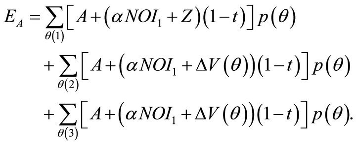
The value of the A note at the end of the period is:

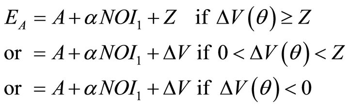(21)

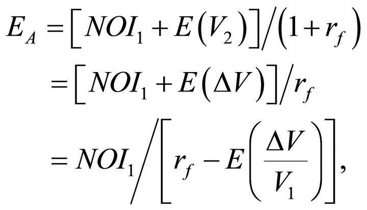
Here A is the principle of the A note and, a function of the state of the world, is the appreciation in value. The appreciation in value exceeds Z in states of the world denoted, the appreciation in value is less than Z in states of the world denoted, and change in value is negative in states of the world. Therefore the value of the A note at the beginning of the period is:

(22)

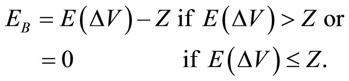
The value of the B note at the end of the period is:

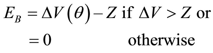(23)

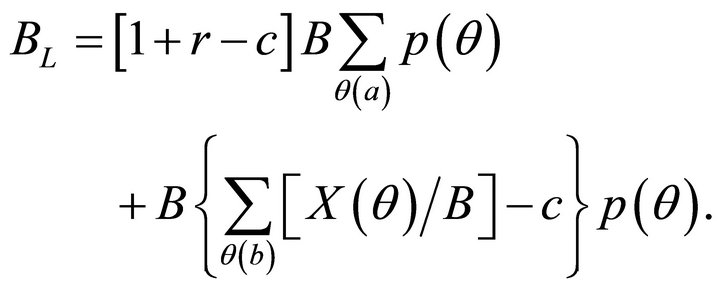
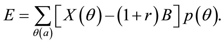
Therefore the value of the B note at the beginning of the period is:

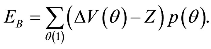(24)

The value of the B note depends upon states of the world and Z, the amount of any appreciation that must be paid to the A note (if appreciation is equal to or exceeds Z).

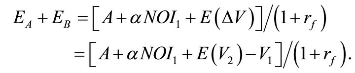
The combined value of the two notes does not depend upon the split into the A and B notes, and is:

(25)

Since all risks can be mitigated,

(26)

If A is set equal to V₁ so that (as evidently it was in the example cited by Yoon [1]), from Equation (19),

and

(27)

Current appraised value includes the present value of any expected appreciation in value. The standard method for appraised value is to divide net operating income by the overall capitalization rate ρ, which equals the riskadjusted cost of capital r minus the expected rate of appreciation in value. It is possible to insure against any risk in this model for purposes of valuing the entire property, so the risk-adjusted cost of capital is replaced by the risk-free rate. Equation (27) shows that the current value of the property takes into account the expected appreciation in value. Since any risk can be insured, the B note has value equal to

(28)

The B note has no value if the A note is allocated the entire value of the property at the time of the creation of the two notes. Evidently such was the case in the Gotham Realty Property example cited by Yoon [1].

Suppose that both the returns to the A and B notes are subject to taxation at rate t. Both interest and capital gains are taxed at the same rate. The value of the A note is now:

(29)

The value of the B note is:

(30)

The value of the two notes is:

(31)

The values are reduced by taxation, but the basic conclusion is still that the B note has value equal to 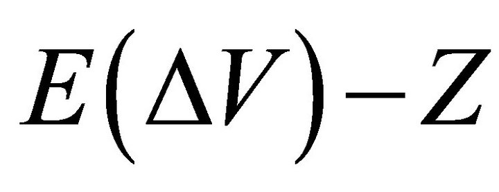if and has no value otherwise.

5. Conclusion

Hope notes are a form of equity participation in defaulted property in which two notes are issued. The A note earns interest and receives repayment of principle and a portion of any appreciation in value, while the B note receives the appreciation in value beyond that due to the holders of the A note. One result in the paper is that the use of this technique has no effect on the value of the property (the sum of the values of the A and B notes). The main result of the paper is that the B note has value only if the expected appreciation in value exceeds the amount of appreciation due to the holders of the A note, and is zero otherwise. In other words, the B note has no value if the A note is, in effect, allocated the entire value of the property at the time the A and B notes are created. Evidently such an allocation occurs frequently, and Yoon (1) cited an example. The paper also shows that the value of the property is reduced by taxation at the entity level. The paper has included the result from McDonald [5] that, if the borrowing rate exceeds the lending rate (as in the case of financial intermediation services), then the value of a firm declines with financial leverage. The value of the firm is reduced by the cost of the financial intermediation services. If the borrowing rate and the lending rates are equal, then the value of the firm is independent of financial leverage, as in Modigliani-Miller Proposition I. This proposition holds in the presence of the possibility of firm bankruptcy.

REFERENCES

- A. Yoon, “Hope Note Strategy Is at Times Hopeless,” Wall Street Journal, Vol. CCLX, No. 278, 2012, p. C3.
- K. Arrow, “The Role of Securities in the Optimal Allocation of Risk Bearing,” Review of Economic Studies, Vol. 31, No. 2, 1963, pp. 61-67.
- J. Stiglitz, “A Re-Examination of the Modigliani-Miller Theorem,” American Economic Review, Vol. 59, No. 5, 1969, pp. 784-793.
- T. Sargent, “Macroeconomic Theory,” 2nd Edition, Academic Press, Orlando, 1987.
- J. McDonald, “The Modigliani-Miller Theorem with Financial Intermediation,” Modern Economy, Vol. 2, No. 2, 2011, 5 Pages.
- F. Modigliani and M. Miller, “The Cost of Capital, Corporation Finance, and the Theory of Investment,” American Economic Review, Vol. 48, No. 3, 1958, pp. 261-297.
- W. Nicholson, “Microeconomic Theory,” 7th Edition, Dryden Press, Orlando, 1998.
- J. McDonald, “Equity Participation: A Theoretical Analysis,” Journal of Real Estate Portfolio Management, Vol. 18, No. 3, 2012, pp. 247-255.