Modern Economy
Vol.4 No.1(2013), Article ID:27494,12 pages DOI:10.4236/me.2013.41003
A Comparison of Three-Stage DEA and Artificial Neural Network on the Operational Efficiency of Semi-Conductor Firms in Taiwan
1Graduate Institute of International Business, National Taipei University, New Taipei City, Taiwan
2Department of economics, Soochow University, Taipei City, Taiwan
3Department of Information Management, Chaoyang University of Technology, Taichung City, Taiwan
Email: hsiang@mailntpu.edu.tw
Received November 12, 2012; revised December 13, 2012; accepted January 10, 2013
Keywords: Data Envelopment Analysis; Three-Stage DEA; Artificial Neural Network; Semi-Conductor Industry
ABSTRACT
In this study, the data envelopment analysis (DEA), three-stage DEA (3SDEA) and artificial neural network (ANN) are employed to measure the technical efficiency of 29 semi-conductor firms in Taiwan. Estimated results show that there are significant differences in efficiency scores among DEA, 3SDEA and ANN analysis. The advanced setting of the three stages mechanism of DEA does show some changes in the efficiency scores between DEA and ANN approaches. We further find that the environmental factor is still a significant variable to explain technical efficiency in Taiwan, irrespective of whether a DEA, 3SDEA or ANN approach is used.
1. Introduction
In this paper, we compare traditional data envelopment analysis (DEA), three-stage data envelopment analysis (3SDEA) and artificial neural network analysis (ANN) to estimate technical efficiency indices, and to explore the effect of environmental factors (Fried, Lovell, Schmidt and Yaisawarng, 2002) [1] on technical efficiency for policy purposes in the semi-conductor sector. We focus on the efficiency assessment since we believe that efficiency and/or performance will become strategic variables in tackling the increasing competitive pressure and structural changes within this industry. We incorporate an operation mechanism and employ DEA, 3SDEA and ANN approaches to our analysis since we consider that the unpredictability of market demand and supply makes the semi-conductor companies’ input-output relationship vary.
The semi-conductor industry is a promising knowledge-intensive industry, which is characterized by large capital, high-quality talent, longer reward and profit for R & D activities, therefore semi-conductor companies must be accountable for the R & D efforts they provide (Chiesa and Toletti, 2003) [2]. In the 1980s, a push for accountability was undertaken in United States and all semi-conductor companies faced the task of allocating scarce resources among high risk and high return R & D activities. Semi-conductor companies are concerned with efficiency, and current tight economic conditions have further highlighted the importance of those concerns. In the 1990s, Taiwan government declared the Technology Industry Establishment Promotion Decree which emphasized the importance of the semi-conductor industry as critical in the development of Taiwan’s manufacturing industry. The government also included the semi-conductor industry in the ten emerging focus industries in 1998. Under this climate of focus, Taiwan started to increase operational efficiency in the semi-conductor industry, and to place extra funds into the supply market. The objective of this focus was to increase quality of life and reduce financial uncertainty. Taiwan’s semi-conductor companies have also confronted accountability issues in the 2000s with administrators bringing some revolutionary changes.
A semi-conductor firm may be viewed as an enterprise in which the professional staff provides the operating conditions for converting quantifiable resources (inputs) into patents and revenues (outputs). However R & D expense faces budget constraints, and whether or not there is a price tag attached, firms need to choose among competing expenditure options. The efficiency of semiconductor companies is a critical issue in the development of the technology industry while operational inefficiency increases uncertainty owing to fluctuations in the financial environment. The issues of market risk emerge when we evaluate the operating efficiency of semi-conductor companies (Kliger and Sarig, 2000) [3]. Due to the continued rapid improvement of semi-conductor technology, it is expected that logistics management has become an increasingly important segment of the semiconductor industry. Therefore, major issues in this study focus on the effect of factory location as part of the firm’s logistics management, when the carriage cost is viewed as an important input in Taiwan. Changes in the financial and political environment will undoubtedly affect a firm’s location decision.
The research intensity and factory location present a useful reference indicator to the investor and legalistic institution (Garner, 1999) [4]. Thus, incorporating the environmental effects of the research intensity and factory location into the performance evaluating system of semi-conductor companies can obviously improve the effectiveness of the evaluation results because the invisible external and internal environment factors are included in the evaluating system in order to fit actual situations in the semi-conductor companies (Larsen, 2006) [5]. We then employ a three-stage data envelopment analysis method to evaluate semi-conductor company performance in order to tailor the multi-input and multi-output industry setting. To avoid the difficulty in making a subjective choice for the inputs and outputs of the DMUs (decision making unit), the artificial neural network (ANN) can be proposed to choose the inputs and outputs of DMUs which are more related to its operating efficiencies.
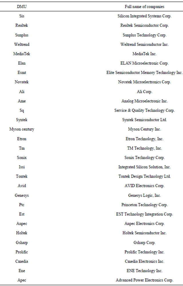
The purpose of this paper is to measure the resource utilization efficiency of semi-conductor companies in Taiwan applying three-stage DEA model and artificial neural network analysis on a sample of 29 semi-conductor companies during the period from 2001 to 2006 (Data sample refers to Appendix 1). This period of data is employed due to avoiding the one-off shock effect in overall efficiency evaluation. Hopefully the empirical results of this study can provide useful information for firms and government agencies to do decision-making about the improvement of operational efficiency.
The reminders of this paper are organized as follows. Section 2 presents a review of the relevant literature. Section 3 describes the methodology of the three-stage DEA and ANN approaches. Section 4 describes the data employed and its characteristics. Section 5 presents the empirical results. The paper then provides the concluding remarks in Section 6.
2. Literature Review
In this section, we firstly introduce the non-parametric programming approach of DEA and the extended 3SDEA to evaluate efficiency and then propose the alternative programming approach of ANN. The DEA approach uses a mathematical programming technique to construct a piecewise linear frontier and it can be referred to as a non-parametric programming approach (Charnes, Cooper and Rhodes, 1978 [6]; Banker, Charnes and Cooper, 1984 [7]). DEA allows researchers to avoid specification of a given functional form or error structure, and many researchers have focused on estimating the technical efficiency and scale efficiency of DMUs by utilizing this technique (Oral and Yolalan, 1990 [8]; Favero and Papi, 1995 [9]; Schaffnit, Rosen and Paradi, 1997 [10]; Fukuyama, Guerra and Weber, 1999 [11]). The DEA model used to evaluate the efficiency in the semi-conductor industry is found in Liu and Wang (2008) [12], Chen and Chen (2007) [13], and Chen and Yeh (2005) [14], while Schaffnit, Rosen and Paradi (1997) [10] present a best practice analysis of bank branches based on a DEA assurance region (DEA-AR) model containing output multiplier constraints, with standard transaction and maintenance times, in order to evaluate allocative efficiency.
The three-stage DEA was first proposed by Fried and Lovell (1990) [15]. Fried, Schmidt and Yaisawarng (1999) [16] then extended three-stage DEA and focused on estimating the environmental variables which influence the input slacks variables. Fried, Lovell, Schmit and Yaisawarng (2002) [1] further compare the efficiency based on the first stage DEA and the third stage DEA; they argue that the three-stage DEA is better than the one-stage DEA adjusting inputs and considering the individual environmental effect and statistical white noise. Greasley (2005) [17] employed a three-stage DEA and simulation to guide operating units to improved performance. The model compared the performance of the current and benchmark process designs. Athanassopoulos and Curram (1996) [18] compared DEA and artificial neural network (ANN) mechanisms to facilitate a definition of efficiency measures from the two methods. Wang (2003) [19] further compared the DEA, stochastic frontier analysis (SFA) and ANN and argued ANN can obtain a similar valid effect of DEA proposed by Charnes, Cooper and Rhodes (1978) [6]. Pendharkar and Rodger (2003) [20] compared the performance of the ANN and DEA by using the “efficient” and “inefficient” training data subsets. It may be useful to screen training data on the screened examples to approximately satisfy the monotonicity property. Liao (2004) [21] proposed an effective procedure on the basis of the artificial neural network (ANN) and the data envelopment analysis (DEA) to optimize the multi-response problems. A case study of improving the quality of hard disk drivers in Su and Tong (1997) [22] is resolved by the proposed procedure and yields a satisfactory solution. Pendharkar (2005) [23] illustrated that a DEA-based data screening of training data improves forecasting accuracy of an ANN using real-world health care and software engineering data. Santin (2008) [24] showed how ANN is a valid semiparametric alternative for fitting empirical production functions and measuring technical efficiency. For the application of ANN in the semi-conductor industry, some results are shown in Wang, Su and Hsieh (2007) [25] and Buddefeld, Grosspietsch, Hosticka and Klinke (1991) [26]. These results demonstrate that DEA-ANN methods offer an useful range information regarding the assessment of performance.
This paper then extends the basic deterministic DEA method to incorporate the three-stage DEA mechanism in order to obtain a more similar comparison base between artificial neural network programming and three-stage DEA approaches.
3. The Three-Stage DEA and ANN Approaches
3.1 Three-Stage DEA Approach
In the DEA approach, Charnes, Cooper and Rhodes (1978) [6] initiated the data envelopment analysis method. They proposed an operational framework for the estimation of productive efficiency (the CCR model) which demonstrated that the mechanism for calculating DEA scores can be formulated as a linear programming problem. We denote  as the n-th output of the j-th DMU and
  as the m-th input of the j-th DMU. If a DMU employs M inputs to produce N outputs, the score of j-th DMU, Ej, is a solution from the linear programming problem,
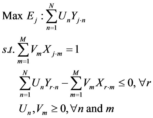
where  and Un and Vm give the weights associated with each output and input. The technical efficiency of each DMU is calculated by using the ratio of a weighted sum of output to a weighted sum of input. Here the input usage of a DMU is radial contracted to the best practice frontier (i.e., isoquant), and the DMU is assumed to continue using its original production process (i.e., production ray). The distance between the actual performance of the DMU and the best-practice frontier provides a measure of the relative inefficiency of the DMU. The DEA best-practice frontier is constructed from piecewise linear combinations of all available DMUs with each DMU being assigned a positive weight when constructing the bestpractice frontier of the N-th DMU. DMUs with positive weights are used to construct the best-practice frontier and a unique set of weights is determined when calculating the efficiency for each DMU. These weights generate the theoretical best-practice DMU, against which a DMU is compared when calculating that particular DMU’s technical efficiency. The weights assigned to the DMUs in order to calculate the technical efficiency of the N-th DMU are then used to calculate the cross-efficiencies of the remaining N-1 DMUs, if necessary. Notably, the pure technical efficiency can be derived through the condition of variable returns to scale. We can add
  to the former model to make the famous BCC model (Banker, Charnes and Cooper, 1984) [7], which provides valuable information about the cost-benefit evaluation. We can calculate the pure technical efficiency score from the BCC model, and then the scale efficiency score can be derived from the technical efficiency and pure technical efficiency scores in that the technical efficiency score is equal to the multiplication of pure technical efficiency and scale efficiency scores (Fare, Grosskopf and Lovell, 1985) [27].
We employ the three-stage DEA model (Fried, Lovell, Schmidt and Yaisawarng, 2002) [1] in order to decompose the environmental and statistical noise effects from the efficiencies and further estimate the real efficiency of each DMU. Under this consideration, it can obtain an objective operating efficiency measure given the identical external environment conditions.
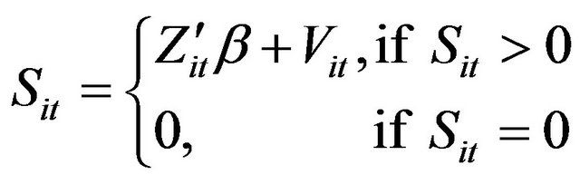
In the first stage, we employ the DEA method together with the output and input variables to estimate the efficiency values and also obtain input slacks given that the environmental variables are controlled; a type of deterministic model where the statistical noise is still allowed. As to the second stage, let the dependent variable be the slack variable on each factor input, and the independent variable be the environmental variable. We can set up four types of regressions on the input slack variables as follows,
 (6)
(6)
where  represents the slack value of each input of i-th DMU within period at
  Z is the vector
  and the first element is set as one. Comparing to the intercept item, other k − 1 elements represents the environmental variable of i-th, and
  is the corresponding coefficient vector and
  is the random error item. We can estimate Equation (6) by the Tobin fixed effect model with the pooled data, and obtain the consistency estimator of coefficient estimate. Thus, we can divide the effect on the input variables into the environmental variables, managing X-inefficiency, and random error item. Based on the method of adjusted input variable suggested by Fried et al. (2002) [1], one can keep each DMU facing the identical operating environment and opportunity by way of uplifting the data of input variables. The adjusted equation is shown as follows:
 (7)
(7)
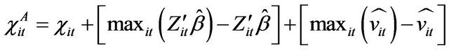
where  represents the t-th adjusted data of specific input variable of i-th DMU and
  represents the originnal data of specific input variable of i-th DMU.
 is the maximal fitted value within the whole sample, representing the worst operating environment, and vice versa. Similarly,
  is the largest residual within the whole sample, representing the worst fortune and/or opportunity, and vice versa. If the coefficient of environmental variables is negative in the regression on the input slack variable, it represents the beneficial managing environment, given that it can reduce the factor surplus in the sample business. Similarly, firms with smaller residuals represent that it encountered good luck and results in a reduction of the factor surplus. In this circumstance, each DMU faces an identical managing environment in order to reflect the actual operating efficiency through the adjustment of the second stage.
In the third stage, we employ the original DEA model to estimate the operating efficiency by way of the adjusted input variable from the second stage and the original output value from the first stage. It other words, we repeat the procedure of the first stage except that we use the adjusted input variable from the second stage (Equation (7)). At this time, we have decomposed the effects on the environmental conditions and statistical noise effects from efficiencies and obtain the real efficiency of each decision making unit. Notably, Fried, Schmit and Yaisawarng (1999) [16] and Fried, Lovell, Schmit and Yaisawarng (2002) [1] recognize that a firm’s technical efficiency will be influenced by the outside environment. They suggest that one should evaluate the effect on the change of input slack variable by the environment variable.
3.2 The ANN Approach
Alternatively, the artificial neural network analysis (ANN) is concerned with the simple simulation or training function base, and focuses on an establishment of the training sample based on previous experience under the assumption that back-propagation network mechanism based on rational economic behavior. In general, ANN model or procedure is specified by network topology, node characteristics and training or learning rules. It is an interconnected set of weights that contains the information or knowledge generated by the model. There are many varieties of connections under study; here in our study we discuss only one type of network which is called the multilayer perception (MLP). The composition of MLP has three main components: input layer, hidden layer and output layer, and can be illustrated in Figure 1.
In this study, as it is explained later, the DMU evaluation variables such as number of stuff employed (NSE), expense of fixed assets (EFA), R & D expenses (RD), net business revenues (NBR), ratio of income before tax (RI) and earnings per share (EPS) are defined as the components (Xj) in input layer of ANN system, the technical efficiency which generated according to DEA results are defined as the components (Yj) in output layer.
Our ANN is composed of a large number of simple processing units, each interacting with others via excitatory or inhibitory connection (Figure 1). Distributed rep-
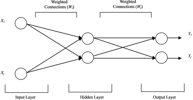
Figure 1. Framework of ANN (Xj refers to input values and Yj refers to output values).
resentation over a large number of unit together with interconnectedness among processing units, provide an error tolerance. Three different layers can be distinguished. The input layer is responsible for receiving information from the outside environment and transferring it to the hidden layer. In the hidden layer, a neuron will assign a series of weights to the input, cope with the information via a training process, and then forward the results with weights to the output layer.
As indicated in Figure 1, a typical three-layer feedforward model used for forecasting purposes. In this study, the input nodes are the observations of NSE, EFA, RD, NBR, RI and EPS while the output provides the forecast for the future values of efficiencies for DMUs. Hidden nodes with appropriate nonlinear transfer functions are used to process the information received by the input nodes. The MLP’s most popular learning rule is the error back-propagation algorithm. Back-propagation learning is a kind of supervised learning introduced by Werbos (1974) [28] and later developed by Rumelhart and McClelland (1986) [29]. The algorithm uses a learning set, which consists of input desired output pattern pairs. Each input-output pair is obtained by the offline processing of historical data. These pairs can be used to adjust the weights in the network to minimize the mean squared error (MSE) which measures the difference between the real and the desired values over all output neurons and all learning patterns. After computing MSE, the back-propagation step computes the corrections to be applied to the weights. Under this process we determine how close the actual output to new situations is. In the learning process the values of interconnection weights are adjusted so that the network produces a better approximation of the desired output.
According to this procedure, the values of intercomnection weights related to inputs, outputs and their efficiency scores of each DMUs can be obtained. Since the structure of ANN is suitable to made concave functions with multidimensionality, therefore it can be used in creating efficient frontier functions and estimating efficiencies of DMUs (Wang, 2003) [19]. Based on this network design and process, we can farther compute the efficiency scores of each DMUs through the inputs and outputs which have the relative higher value of interconnecttion weights.
4. The Data
We employ the institution functions of the firm in this paper, which is in line with the competitive semi-conductor industry in Taiwan. This can also effectively benefit a firm’s operations and improve a semi-conductor firm’s efficiency. In accordance with this approach, we specify three types of firm’s output, namely the net business revenues (business revenues after tax), ratio of gross income before tax, ratio of net income after tax, ratio of business profit, turnover of accounts payable, and earnings per share. The first four types of output constitute the main activities of semi-conductor firms; with the last two representing an extended source of revenue for firms (Chiesa and Toletti, 2003) [2]. The input measures based on the above output entail operating resources. We select the following three input factors: number of staff employed, expense of fixed assets, and R & D expenses.
It should also be noted that the ratio of net income after tax is sourced as a ratio of gross income before tax, the ratio of net income after tax being their main element. One of these needs to be excluded in order to avoid a multicollinearity problem in the DEA model. The results of our correlation analysis also support the high correlation phenomenon between these two variables, with a correlation coefficient of 0.919. We then choose the ratio of net income before tax for further analysis.
Next, we determine the relationships between inputs and outputs. The DEA model requires definitions of inputs and outputs so that when inputs are added, outputs will increase. We employ a correlation analysis to test for isotonicity (i.e., the positive direction of the relationship between inputs and outputs). According to the results of the inter-correlation analysis, it is clear that the correlation coefficients between our chosen outputs and inputs are all positive.
Third, we have further utilized correlation analysis to determine the appropriate inputs/outputs in accordance with this approach (Golany and Roll, 1989) [30]. The less correlation between inputs and outputs is neglected since it is weak production oriented. Ratio of business profit and turnover of accounts payable are excluded in the further analysis. Thus, we specify three types of firm output, namely net business revenues (NBR), ratio of gross income before tax (RI) and earnings per share (EPS). Three types of input, namely number of staff employed (NSE), expense of fixed assets (EFA), and R & D expenses (RD) are included. The summaries of the data are provided in Table 1.
The official report from the Commission on National Corporations of the Ministry of Economic Affairs provides a rich source of data on the operations of all of Taiwan’s semi-conductor firms. We have gathered the requisite data for 29 companies, which represent 90 per cent of the domestic companies in Taiwan, covering the period 2001 to 2006. Please note that we chose the time span of 2001 to 2006 because the Taiwanese government first included the semi-conductor industry into the ten emerging important industries in 2000 and we evaluated the promotion performance in the first six-year periods. We employed MATLAB 7.0 software to solve the artificial neural network programming problem and we used Frontier-41 software to run the three-stage DEA analysis.
5. Empirical Results
5.1 The Mean of Efficiency Values in the DEA, Three-Stage DEA and ANN
As indicated in Table 2, we can observe that the calculated mean technical efficiency between 2001 and 2006 was 0.825 by traditional DEA. Relative to their production frontier, semi-conductor companies operated efficiently with actual activities 20% above the maximum activity levels during 2001-2006. As for technical efficiency in each year, we then find that it was 0.866 in 2001, with a gentle uplift to 0.892 in 2002, and 0.911 in 2003, followed by a steep decline to 0.844 in 2004. It is clear that average technical efficiency slumped in 2005 (0.708) relative to 2004. We also find that the mean technical efficiency score of 0.708 and 0.732 during the period 2005-2006 was lower than during the periods 2001-2004, at 0.866, 0.892, 0.911, and 0.844 respectively. The technical efficiency score (TE) equals the product of the pure technical efficiency (PTE) and the scale efficiency (SE) scores, and the relative magnitudes of these scores provide evidence of the source of the inefficiencies. Similar results can be found when PTE and SE scores are analyzed. The PTE score of 0.972, 0.944, 0.973 and 0.933 over the period 2001 to 2004 was also higher than the 0.759 in 2005 and 0.829 in 2006; while the SE scores of 0.891, 0.945, 0.936, 0.905 during the period 2001 to 2004 were not higher than the 0.933 and 0.833 in 2005-2006.
We further find that the mean pure technical efficiency scores of semi-conductor companies (0.901) were lower than the mean scale efficiency score (0.915) during the 2001 to 2006 period. This seems to suggest that pure technical inefficiency has a greater significance than scale inefficiency as a source of inefficiency within all inefficient semi-conductor companies. Thus, given input prices, the effects on technical inefficiency could be attributed to the inappropriate incorrect choice of the initial input combinations, rather than the returns of scale. The reason is that semi-conductor companies increase their own scope or mass investment, and that the resource allocation issue is neglected. Semi-conductor companies suffer higher operating costs on the account that they produce goods without optimal production efficiency. Similar results can be found when periods of data are used for 2005 to 2006, with the respective mean pure technical efficiency scores (0.759; 0.829) being lower than the respective mean scale efficiency scores (0.933; 0.883).
The mean technical efficiency scores of an ANN ap-
Table 1. Summary of the descriptive statistics of the input and output data.
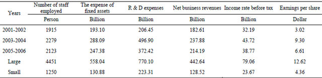
Note: All monetary values are in NT$ billion. The data consists of thirty-nine domestic commercial semi-conductor companies and the seven years’ data. The data consists of seven large-sized semi-conductor companies, and twenty-two small-sized semi-conductor companies.
Table 2. The mean of efficiency values in the DEA, three-stage DEA and ANN during the year of 2001-2006.
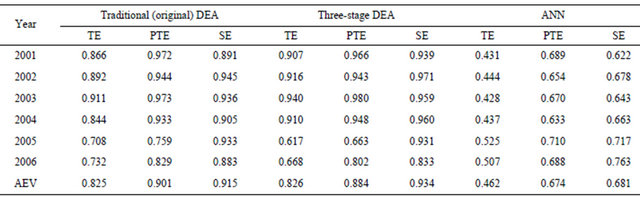
Notes: TE: technical efficiency; PTE: pure technical efficiency; SE: scale efficiency; AEV: average efficiency value. The results of sensitivity analysis of year 2001 data are reported here, and the similar results are also obtained when 2001-2007 data are employed.
proach in Table 2 is 0.462, implying that semi-conductor companies could have produced the same level of output using 46% of the input actually used. Using the threestage DEA approach, we find that the three-stage DEA efficiency scores (0.826) are on average higher than that of ANN scores (0.462). Similar results are also obtained when the regular DEA technical efficiency is employed. The three-stage frontier (and/or traditional DEA frontier) of semi-conductor companies is naturally a “soft” frontier, at which the output observations of semi-conductor companies are in some cases allowed to cross the envelope, allowing us to make more observations closer to this frontier. However, the ANN frontier is a “hard” frontier for any given figures, and the envelope is located far from the three-stage frontier. Hence, the three stage DEA frontier may be crossed by a few efficient semiconductor companies, but most semi-conductor companies (95% or more) are still assumed to fall on or beneath the frontier. That is, the efficiency scores of 3SDEA are higher than ANN. Similar results are also obtained when pure technical efficiency and scale efficiency are analyzed. We further find that the average pure technical efficiency and scale efficiency are 0.674 and 0.681 from the artificial neural network analysis (ANN), which are significantly lower than the result gained from the threestage DEA approach (0.884; 0.934), or the traditional DEA (0.901; 0.915) (Table 2).
We then employ a Tobit regression model in the second stage in order to obtain a consistency estimator by solving the intercept issue of data. The intercept issue of data occurred due to the value of slack variables being less than zero, which is not permitted. As indicated in the second column in Table 3, we find that there are positive and significant coefficients in a number of semi-conductor companies’ location. There is also a positive result for R & D intensity and the slack variable of the number of staff employed; it shows that the input of the number of staff employed should increase; however, it does not need to be adjusted constantly due to the negative and insignificant coefficient displayed by the number of years that the business has been run for. As to the third column in Table 3, the inputs of R & D expenses should increase because there are positive and significant coefficients in a number of semi-conductor companies’ location, and R & D intensity in the regression of the slack variable of R & D expense. Additionally, there is a negative and significant coefficient of establishment years in the regression of the slack variable of R & D expense. It shows that more years of establishment is beneficial to the semi-conductor companies in order to deduce the extraneous inputs of R & D expense. The decrease in the inputs of R & D expense is attributed to a benevolent operating environment. Additionally, as to the second columns in Table 3, the inputs of fixed assets and R & D expense should be increase especially when the company operates in more than one country because there are positive and significant coefficients of location in the regressions of the slack variable of fixed asset and R & D expense; however, one does not adjust the fixed asset and R & D expense due to the insignificant coefficients of the number of semi-conductor companies location, and establishment years on the slack variable of personnel expense.
Based on the estimated adjusted inputs from the second stage and the original outputs from the first stage, we can estimate the technical efficiency again using DEA. Among the estimated technical efficiency in this stage, one can reflect the actual operating efficiency, representing the results on the removal of the environmental factor and statistical noise effects. Table 4 lists the polished efficiency of the 29 semi-conductor companies in Taiwan.
5.2 Testing Efficiency Differences for DEA, Three-Stage DEA and ANN Approach
Based on Table 4, our results are identical with those of Fried, Lovell, Schmit and Yaisawarng (2002) [1]. The
| |
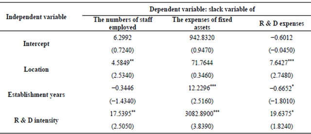
Notes: ***, **, *Representing the significance of 1%, 5%, 10%, respectively. Log likelihood = −595.6005.
Table 4. Numbers of semi-conductor companies with efficient efficiency and economies of scale during 2001-2006.
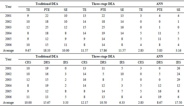
Notes: TE: technical efficiency; PTE: pure technical efficiency; SE: scale efficiency; AEV: average efficiency value. CRS = constant return to scale; DRE = decreasing returns to scale; IRS = increasing returns to scale.
number of efficient semi-conductor companies, with the technical efficiency that equals unity, is higher during the three-stage DEA (13 DMUs) than that of the first stage DEA (9 DMUs) in 2001. Similar results are also obtained when scale efficiency is analyzed. We further find that the majority of sample semi-conductor companies belong to the stage of decreasing returns to scale (DRS). The number of firms with constant returns to scale during 2001- 2006, is also higher during the three-stage DEA (12.17 DMUs) than that of the first stage DEA (10.00 DMUs).
The percentage of decreasing returns to scale firms during 2001-2004 is 65.5%, 55.2%, 51.7%, and 65.4% respectively. The source of the inefficient semi-conductor companies mostly arise from scale inefficiency. Similar results are also obtained when 2005-2006 data is analyzed. We can derive that the semi-conductor companies are shifting from decreasing returns to scale (DRS) to increasing returns to scale (IRS) through the adjustment of the effects on the environment and rand effort in the three-stage DEA. This implies that the production scale of the firms have adjusted and are close to the optimum scale.
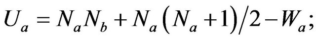
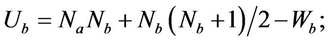
Two Banker’s asymptotic DEA efficiency tests have been used to test for inefficiency differences between two different efficiency scores (Banker, 1996 [31];
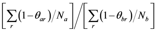
Banker and Chang, 1995) [32]. Firstly, we assume that the two inefficiencies  follow the exponential distribution. The test statistic

is evaluated relative to the F-distribution with (2Na, 2Nb) degrees of freedom. Secondly, we assume that the two inefficiencies  follow the half-normal distribution. The test statistic
is evaluated relative to the F-distribution with  degrees of freedom. Another two traditional test procedures, Welch’s mean test and Mann-Whitney test have also been used to test for comparison on inefficiency differences between the different efficiency scores. For Welch’s mean test, the test statistic, under the assumption of unequal variances, is given by,
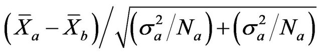
which follows the t-distribution of freedoms calculated as,

where  and
and  and
and  and
and  are the sample means and variances of the inefficiencies. In the MannWhitney test, the test statistic Z-value is calculated by
and  is the lower figure between the calculated magnitudes of
  and
and ,
,
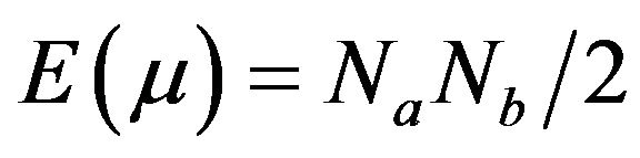
and
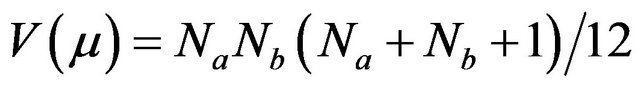
where  and
and  are the rank sums of each selected sample. In our case, one of N has large sample sizes (N > 15); we can generate a Z-value and refer to the standardized normal distribution to test the null hypothesis.
We apply four tests: Banker’s two asymptotic DEA tests, Welch’s mean test and Mann-Whitney test in our study. All tests show that there is a significant difference among the average efficiency scores of ordinary DEA vs. ANN methods (see the third column, Table 5), and 3SDEA versus ANN methods (see the fourth column, Table 5). Moreover, the advanced setting of the threestages mechanism of DEA does not change the instincttive differences of DEA mechanisms. Derived results can be obtained when DEA and 3SDEA are compared and efficiencies obtained within these two approaches are not different as confirmed in four kinds of tests (see the fifth column, Table 5). Estimated results show that there are significant differences in efficiency scores between three-stage DEA and ANN. Similar results are also obtained when the efficiencies of regular DEA and ANN are compared. Identical to the results of Fried, Lovell, Schmit and Yaisawarng (2002) [1], we find that different approaches (DEA versus ANN) will result in different results when they are employed in similar methodologycal framework. The advanced setting of the three-stage mechanism of DEA does not change the instinctive differences between DEA and ANN approaches.
6. Concluding Remarks
In this study, ordinary (original) DEA, three-stage DEA, and artificial neural network (ANN) approaches are employed to compare the technical efficiency of 29 semiconductor companies in Taiwan. The six-year data set 2001-2006 is employed, which avoids the one-off shock effect in the overall efficiency evaluation. Estimated results show that there are significant differences in efficiency scores between three stages DEA and ANN. Similar results are also obtained when the efficiencies of regular DEA and ANN are compared. Identical to the results of Fried, Lovell, Schmit and Yaisawarng (2002) [16], we find that different approaches (DEA vs. ANN) will produce different results when they are employed in similar methodological framework. Furthermore, the advanced setting of the three-stage mechanism of DEA does not change the instinctive differences between DEA and ANN approaches. The results are comparable as a whole; however, ANN approach produces a more robust frontier and identifies more efficient units since more good performance patterns are explored. Furthermore, ANN approach provides worse performers the guidance on how to improve their performance in different efficiency ratings. The neural network approach requires no assumptions about the production function (the major drawback of the parametric approach) and it is highly flexible.
We also find that the environmental factors still provide a significant variable to explain the technical efficiency in the efficiency model, irrespective of whether DEA, 3SDEA or ANN approach is employed. Nevertheless, future research with neural networks in the efficiency analysis is suggested. The possible directions include weight restrictions and cross-industry comparesons and, etc.
Table 5. Summaries of efficiency difference test results.
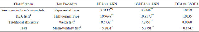
Notes: 1). **Represents significance at the 0.05 level and *represents significance at the 0.10 level. 2). As to semi-conductor’s asymptotic DEA tests, there are six tests performed: the exponential type, a) DEA vs. ANN (=0.3943/0.1191 = 3.3112), b) 3SDEA vs. ANN (=0.3943/0.1193 = 10.9170), c) DEA vs. 3SDEA (=0.1193/0.1191 = 1.0018); the half-normal type, d) DEA vs. ANNA (=0.1554/0.0142 = 10.9649), e) 3SDEA vs. ANN (=0.1554/0.1423 = 10.9170), f) DEA vs. 3SDEA (=0.0142/0.0141 = 1.0035). 3). As to Welch efficiency tests, there are also three tests performed: a) DEA vs. ANN (=0.2752/0.0321 = 8.5732), b) 3SDEA vs. ANN (=0.2750/0.0378 = 7.2751), c) DEA vs. 3SDEA (=0.0002/0.0331 = 0.0060). 4). As to Mann-Whitney efficiency tests, there are also three tests performed, that is, a) DEA vs. ANN of technical efficiency ((490 − 495) − 162)/31.61 = −5.2831, b) 3SDEA vs. ANN of technical efficiency ((−27 − 162)/31.61 = −5.9791), c) DEA vs. 3SDEA of technical efficiency ((135 − 162)/31.61 = −0.8542). Note that 162 and 31.61 are the calculated average and the standard deviation of the selected sample.
Based on the analytical results, the semi-conductor companies in Taiwan should take output factors and the business environment as important factors for improving operating performance. The empirical results also show that the three-stage DEA efficiency is different from the ordinary (first stage) DEA efficiency. Each semi-conductor company of average technical efficiency and scale efficiency in the three-stage DEA is better than in the first stage DEA. Compared with the first stage DEA, the numbers of semi-conductor companies for technical efficiency and scale efficiency values which are equal to one increased. The development of the business environment can enhance technical and scale efficiencies. To decompose environmental and statistical noise effects from efficiencies could estimate real efficiency of every decision making unit. The conclusions of these empirical results may provide some information to identify not only the efficiency of semi-conductor companies but also give evidence to promote the operating efficiency via adapting or adjusting the effects of environmental situations as indicated in this article.
REFERENCES
- H. O. Fried, C. A. K. Lovell, S. S. Schmidt and S. Yaisawarng, “Accounting for Environmental Effect and Statistical Noise in Data Envelopment Analysis,” Journal of Productivity Analysis, Vol. 17, No. 1, 2002, pp. 157-174. doi:10.1023/A:1013548723393
- V. Chiesa and G. Toletti, “How Biotechnology Changes Pharma R & D: A Managerial Perspective,” International Journal of Biotechnology, Vol. 5, No. 2, 2003, pp. 125-136.
- D. Kliger and O. Sarig, “The Information Value of Bond Ratings,” The Journal of Finance, Vol. 6, No. 12, 2000, pp. 2879-2902.
- B. A. Garner, “Black’s Law Dictionary,” West Publishing Co., New York, 1999.
- P. T. Larsen, “Merrill’s Dublin-Based Financial Holding Company Is Planning to Expand in Areas,” Financial Times, Vol. 10, No. 1, 2006, pp. 15-16.
- A. Charnes, W. W. Cooper and E. Rhodes, “Measuring the Efficiency of Decision Making Units,” European Journal of Operational Research, Vol. 2, No. 12, 1978, pp. 429- 444. doi:10.1016/0377-2217(78)90138-8
- R. D. Banker, A. Charnes and W. W. Cooper, “Some Models for Estimation of Technical and Scale Inefficiencies in Data Envelopment Analysis,” Management Science, Vol. 30, No. 12, 1984, pp. 1078-1092.
- M. Oral and R. Yolalan, “An Empirical Study on Measuring Operating Efficiency and Profitability of Bank Branches,” European Journal of Operational Research, Vol. 46, No. 2, 1990, pp. 282-294.
- C. A. Favero and L. Papi, “Technical Efficiency and Scale Efficiency in the Italian Banking Sector,” Applied Economic, Vol. 27, No. 3, 1995, pp. 385-395. doi:10.1080/00036849500000123
- C. Schaffnit, D. Rosen and J. C. Paradi, “Best Practice Analysis of Bank Branches: An Application of DEA in a Large Canadian Bank,” European Journal of Operational Research, Vol. 98, No. 2, 1997, pp. 269-289. doi:10.1016/S0377-2217(96)00347-5
- H. Fukuyama, R. Guerra and W. L. Weber, “Efficiency and Ownership: Evidence from Japanese Credit Cooperatives,” Journal of Economics and Business, Vol. 51, No. 4, 1999, pp. 473-487. doi:10.1016/S0148-6195(99)00020-X
- F. H. F. Liu and P. H. Wang, “DEA Malmquist Productivity Measure: Taiwanese Semi-Conductor Companies,” International Journal of Production Economics, Vol. 112, No. 1, 2008, pp. 367-376. doi:10.1016/j.ijpe.2007.03.015
- T. Y. Chen and L. H. Chen, “DEA Performance Evaluation Based on BSC Indicators incorporated: The Case of Semi-Conductor Industry,” International Journal of Productivity and Performance Management, Vol. 56, No. 4, 2007, pp. 335-357.
- C. J. Chen and Q. J. Yeh, “A Comparative Performance Evaluation of Taiwan’s High-Tech Industries,” International Journal of Business Performance Management, Vol. 7, No. 1, 2005, pp. 16-32. doi:10.1504/IJBPM.2005.006241
- G. D. Ferrier and C. A. K. Lovell, “Measuring Cost Efficiency in Banks: Econometric and Linear Programming Evidence,” Journal of Econometric, Vol. 46, No. 2, 1990, pp. 229-245. doi:10.1016/0304-4076(90)90057-Z
- H. O. Fried, S. S. Schmidt and S. Yaisawarng, “Incorporating the Operating Environment into a Nonparametric Measure of Technical Efficiency,” Journal of the Productivity Analysis, Vol. 12, No. 2, 1999, pp. 249-267. doi:10.1057/palgrave.jors.2601857
- A. Greasley, “Using DEA and Simulation in Guiding Operating Units to Improved Performance,” The Journal of the Operational Research Society, Vol. 5, No. 6, 2005, pp. 727-740.
- A. D. Athanassopoulos and S. P. Curram, “A Comparison of Data Envelopment Analysis and Artificial Neural Networks as Tools for Assessing,” Journal of the Operational Research Society, Vol. 47, No. 8, 1996, pp. 100-117.
- S. H. Wang, “Adaptive Non-Parametric Efficiency Frontier Analysis: A Neural-Network-Based Model,” Computers & Operations Research, Vol. 30, No. 2, 2003, pp. 279- 296. doi:10.1016/S0305-0548(01)00095-8
- P. C. Pendharkar and J. A. Rodger, “Technical EfficiencyBased Selection of Learning Cases to Improve Forecasting Accuracy of Neural Networks under Monotonicity Assumption,” Decision Support Systems, Vol. 36, No. 1, 2003, pp. 117-136. doi:10.1016/S0167-9236(02)00138-0
- H. C. Liao, “A Data Envelopment Analysis Method for Optimizing Multi-Response Problem with Censored Data in the Taguchi Method,” Computers & Industrial Engineering, Vol. 46, No. 4, 2004, pp. 817-835. doi:10.1016/j.cie.2004.05.012
- C. T. Su and L. I. Tong. “Multi-Response Robust Design by Principal Component Analysis,” Total Quality Management, Vol. 8, No. 3, 1997, pp. 409-420. doi:10.1080/0954412979415
- P. C. Pendharkar, “A Data Envelopment Analysis-Based Approach for Data Preprocessing,” IEEE Transactions on Knowledge & Data Engineering, Vol. 17, No. 10, 2005, pp. 1379-1388. doi:10.1109/TKDE.2005.155
- D. Santin, “On the Approximation of Production Functions: A Comparison of Artificial Neural Networks Frontiers and Efficiency Techniques,” Applied Economics Letters, Vol. 15, No. 7, 2008, pp. 597-600. doi:10.1080/13504850600721973
- J. T. Wang, C. T. Su and H. T. Hsieh, “A Framework for Determining MIMO Process Parameters by a Neuro-DM & ACO Approach,” International Journal of Production Research, Vol. 45, No. 15, 2007, pp. 350-365.
- J. Buddefel, K. E. Grosspietsch, B. J. Hosticka, R. Klinke and G. Wagner, “An Intelligent Sensor Integrated Preprocessing Facility for Neural Networks,” Microprocessing and Microprogramming, Vol. 32, No. 3, 1991, pp. 335- 342. doi:10.1016/0165-6074(91)90367-3
- R. Fare, S. Grosskopf and C. A. K. Lovell, “The Measurement of Efficiency of Production,” Kluwer Academic Publishers, Boston, 1985.
- P. I. Webos, “Beyond Regression: New Tools for Prediction and Analysis in the Behavior Science,” Ph.D. Thesis, Harvard University, Cambridge, 1974.
- D. E. Rumelhart and J. L McClelland, “Parallel Distributed Processing: Exoloration in the Microstructure of Cognition,” MIT Press, Cambridge, 1986.
- B. Golany and Y. Roll, “An Application Procedure for DEA,” Omega, Vol. 17, No. 3, 1989, pp. 237-250. doi:10.1016/0305-0483(89)90029-7
- R. D. Banker, “Hypothesis Tests Using Data Envelopment Analysis,” Journal of Productivity Analysis, Vol. 7, No. 1, 1996, pp. 139-159. doi:10.1007/BF00157038
- R. D. Banker and H. Chang, “A Simulation Study of Hypothesis Tests for Differences in Efficiencies,” International Journal of Production Economic, Vol. 39, No. 1-2, 1995, pp. 37-54. doi:10.1016/0925-5273(94)00061-E
Appendix 1: Data samples of the study