Smart Grid and Renewable Energy
Vol.4 No.6(2013), Article ID:36706,9 pages DOI:10.4236/sgre.2013.46051
Forecasting the Demand of Short-Term Electric Power Load with Large-ScaleLP-SVR
![]()
1Department of Computer Science, School of Engineering and Computer Science, Baylor University, Waco, USA; 2Department of Electrical and Computer Engineering, Autonomous University of Ciudad Juárez (UACJ), Ciudad Juárez, México; 3Science Applications International Corporation, El Paso, USA.
Email: pablo_rivas_perea@baylor.edu, jcota@uacj.mx, dagarcia@uacj.mx, abquezad@uacj.mx, fenrique@uacj.mx gerardo_rosiles@yahoo.com
Copyright © 2013 Pablo Rivas-Perea et al. This is an open access article distributed under the Creative Commons Attribution License, which permits unrestricted use, distribution, and reproduction in any medium, provided the original work is properly cited.
Received November 13th, 2012; revised January 5th, 2013; accepted January 12th, 2013
Keywords: Power Load Prediction; Linear Programming Support Vector Regression; Neural Networks for Regression; Bagged Regression Trees
ABSTRACT
This research studies short-term electricity load prediction with a large-scalelinear programming support vector regression (LP-SVR) model. The LP-SVR is compared with other three non-linear regression models: Collobert’s SVR, FeedForward Neural Networks (FFNN), and Bagged Regression Trees (BRT). The four models are trained to predict hourly day-ahead loads given temperature predictions, holiday information and historical loads. The models are trained onhourly data from the New England Power Pool (NEPOOL) region from 2004 to 2007 and tested on out-of-sample data from 2008. Experimental results indicate that the proposed LP-SVR method gives the smallest error when compared against the other approaches. The LP-SVR shows a mean absolute percent error of 1.58% while the FFNN approach has a 1.61%. Similarly, the FFNN method shows a 330 MWh (Megawatts-hour) mean absolute error, whereas the LP-SVR approach gives a 238 MWh mean absolute error. This is a significant difference in terms of the extra power that would need to be produced if FFNN was used. The proposed LP-SVR model can be utilized for predicting power loads to a very low error, and it is comparable to FFNN and over-performs other state of the art methods such as: Bagged Regression Trees, and Large-Scale SVRs.
1. Introduction
Accurate load predictions are critical for short term operations and long term utilities planning. The load prediction impacts a number of decisions (e.g., which generators to commit for a given period of time) and broadly affects wholesale electricity market prices [1]. Load prediction algorithms also feature prominently in reducedform hybrid models for electricity price, which are some of the most accurate models for simulating markets and modeling energy derivatives [2].
Traditionally, utilities and marketers have used commercial software packages for performing load predictions. The main disadvantage of these is that they offer no transparency into how the predicted load is calculated. They also ignore important information, e.g., regional loads and weather patterns. Therefore, they do not produce an accurate prediction.
The general problem of electricity load forecasting has been approached with a combination of support vector machines and simulated annealing with satisfactory results [3] when compared against neural network approaches for regression; however, the problem was not addressed for the particular case of short-term electricity load forecasting. The work by Mohandes [4] represented significant advances in this field by showing that support vector machines over-perform typical statistical approaches and typical neural network algorithms, particularly, the author demonstrate that as the training data increases, the better the performance is for support vector-based classifiers; in spite of this findings, no largescale approaches were tested. Recently, Jain et al. [5] studied the case of clustering the training data with respect to its average pattern and then used support vector machines to forecast power load; the paper reports sampling two years of data to train the support vector machines with outstanding results, nevertheless, no largescale methodologies were used.
To the best of our knowledge, no efforts have been reported to address the problem of short-term electricity load forecasting using a large-scale approach to support vector machines. Our motivation to use a large-scale approach is that such an approach will permit the support vector machine to use a much larger set to define the support vectors that will provide a superior regression performance. Furthermore, we will take advantage of the computational efficiency of a linear programming mathematical formulation for a support vector regression problem. This research considers several variables to build a prediction model and compares results among a Linear Programming Support Vector Regression (LPSVR) approach, a Feed Forward Neural Network (FFNN), and Bagged Regression Trees (BRT). This paper shows that the proposed LP-SVR model provides better forecasts than FFNN and BRT approaches.
2. Dataset
The dataset used for this electricity load prediction problem includes historical hourly temperatures and system loads from the New England Pool region. The original dataset was obtained from the New England ISO. At the time of writing this paper, the direct link to Zonal load data was the one shown in this reference [6]. Table 1 shows the variables included for predicting the electricity load.
These variables are called features. The features to consider are the bulb and dew temperature, the hour of the given day, the day of the week, and whether it is a holiday or weekend. Also, the features include the average load of the previous 24 hours, the lagged load of the previous 24 hours, and the previous week lagged load.
The training set  consists of input feature vectors
  (consistent with the variables listed in Table 1) and targets
  corresponding to the measured electricity load. The total number of training samples is
 . A testing set
  was also used, consisting of
  samples.
Each feature vector  corresponds to one hour reading, i.e., one complete day would be equivalent to 24 sequential feature vectors
 . Consequently, the training set consists of 1461 days, or four years of data. The testing set consists of one leap year of data or 366 days.
3. Training the Regression Models
The regression models will be constructed using the training set . The training procedure involves a training set partition into a new training set and a validation set
 , which is used to auto-adjust model parameters
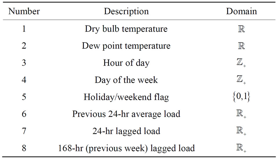
Table 1. Variables used for prediction.
during the learning process. Once the model is trained and internally validated a testing phase follows in order to estimate the true performance errors of the models with unseen data. The complete regression modeling framework is shown in Figure 1.
The actual regression models used in this study are briefly introduced in the following sections.
3.1. Feed-Forward Neural Network
The first regression model used was based on neural networks. In fact, this study uses the Feed-Forward Neural Network architecture because they can approximate any square-integrable function to any desired degree of accuracy provided a training set [7,8]. A simple FFNN contains an input layer and an output layer, separated by l layers (the set of l layers is known as hidden layer) or neuron units. Given an input sample clamped to the input layer, the neuron units of the network compute their parameters according to the activity of previous layers. This research considers the particular neural topology where the input layer is fully connected to the first hidden layer, which is fully connected to the next layer until the output layer.
Given an input feature vector , the value of the
  unit in the
  layer is denoted
 , with
  referring to the input layer,
  referring to the output layer. We refer to the size of a layer as
 . The default activation level is determined by the internal bias
  of that unit. The set of weights
  between
  in layer
  and unit
  in layer
  determines the activation of unit
  as follows:
 (1)
(1)
where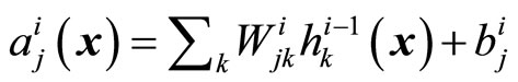 , for all
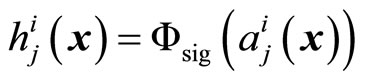
 with
with  and
and  is the sigmoid activation function
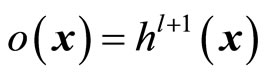
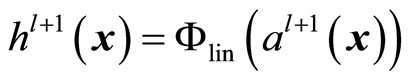
 . Given the last hidden layer, the output layer is computed similarly by
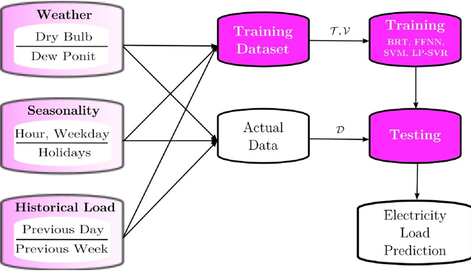
Figure 1. Framework to build regression models for power load prediction. Blocks on the left indicate the input variables, i.e., attributes used to build the regression models.
 (2a)
(2a)
 (2b)
(2b)
where 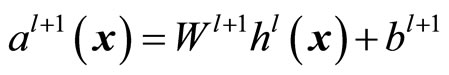 and the activation function
  is of the linear kind which required in regression problems (see text books [9] and [10] for a detailed development). Thus, when an input sample
  is presented to the network, the application of 1) at each layer will generate a pattern of activity in the different layers of the neural network and produce an output with 2). Then
  is the regression output of the neural network.
The FFNN requires a training phase to build the model . In this training phase, we used the “LevenbergMarquardt” algorithm along with with a back-propagation strategy to update the weights
  and biases
 . As a learning function, we used the well established method of gradient descent with momentum weight and bias. The FFNN training phase ends when any of the following conditions holds:
● A number of 100 epochs (i.e. training iterations) is reached;
● The actual mean of absolute error (MAE) is 1 × 10⁻⁶;
● The gradient step size is less than or equal to 1 × 10⁻¹⁰.
A well-established technique for preventing over-fitting in the training was also implemented. This technique consists of partitioning the training set into two sets, training (80%) and validation (20%), such that when the MSE has not been decreased in the past five iterations using the internal validation set, the training phase stops and rolls back to the model  associated with the previous minimum MAE. The network has 20 neurons in the hidden layer, and, as said before, the network uses the mean of absolute error (MAE) metric as the error function to minimize during training.
3.2. Bagged Regression Trees
Bagging stands for “bootstrap aggregation”, which is a type of ensemble learning [11]. The algorithm in general works as follows. To bag a regression tree on a training set , the algorithm generates several bootstrap clones of the training set and grows regression trees on these clones. These clones are obtained by randomly selecting
  samples out of
  with replacement. Then, the predicted response of a trained ensemble corresponds to the average predictions of individual trees [12].
The process of drawing  out of
  samples with replacement omits an average of 37% samples for each regression tree. These are called “out-of-bag” observations. These out-of-bag observations are used as a validation set
  to estimate the predictive power. The average out-of-bag error is computed by averaging the outof-bag predicted responses versus the true responses for all samples used for training. This average out-of-bag error is an unbiased estimator of the true ensemble error and can be used to auto-adapt the learning process [11].
3.3. Large-Scale Support Vector Regression
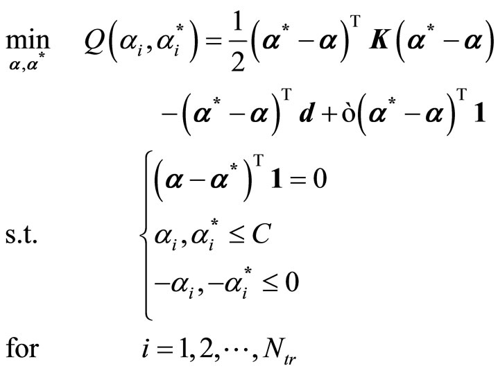
Included in this study is the large-scale support vector regression (LS SVR) training strategy by Collobert, et al. [13], considered the most popular LS-SVR training strategy. Collobert, et al. algorithm is an adaptation of Joachims’ SVM method for SVR problems [13]. The authors reformulate the typical dual SVR problem to have the following Quadratic Programming (QP) minimization problem:
 (3)
(3)
where  is a kernel matrix;
 ’s are the Lagrange multipliers associated with the solution of the problem;
  is the vector of desired outputs, i.e., the targets;
  defines the parameter of the loss function, which represents the amount of deviation from the exact solution that is permitted;
  is the regularization parameter.
Next, the authors perform the same decomposition proposed by Osuna, et al. [14], defining the working set  and the fixed set
 , where the size of the working set is
  with
with . The authors extend Joachims’ idea of the steepest descent direction to select the working set at each iteration of the SVR dual problem [15].As it is known [13], this method also uses a chunking approach, and a shrinking strategy.
3.4. Linear Programming Support Vector Regression
Finally, this study also includes a linear programming (LP) SVR formulation of Rivas et al. [16,17]. The author uses the following SVR optimization problem:
 (4)
(4)
where ’s are the variables that account for the deviations from the actual exact solution to the optimization problem, i.e., they are relaxation parameters.
Since the canonical form of a linear programming problem is the following:
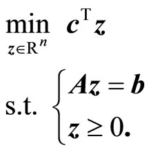 (5)
(5)
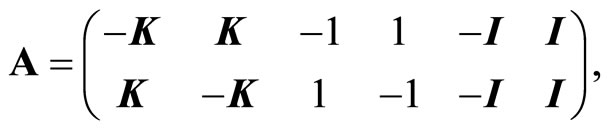
Therefore Problem (4) was posed as a linear programming problem by defining the following equalities:
 (6a)
(6a)
 (6b)
(6b)
 (6c)
(6c)
 (6d)
(6d)
where ,
,  ,
,  , having
  as the vector of variables that contains the unknowns.
Finally, in order to find the solution to the problem, Rivas et al. [16] use a primal-dual interior point methods-based solver to find the variables that satisfy the KKT conditions. The LP-SVR parameters used are ,
,  , and
, and ; these have been found empirically for both this LP-SVR and that SVR by Collobert explained in Section 3.3.
4. Experimental Results
4.1. Experiment Design and Procedure
The experiments consisted of training the four methods with a training dataset 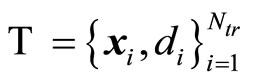 as explained in Section 2. Then the following six error metrics were analyzed using the testing set
 : Mean Absolute Percent Error (MAPE), Mean Absolute Error (MAE), Daily Peak MAPE (DPM), Normalized Error (NE), Root Mean Squared Error (RMSE), and Normalized Root Mean Squared Error (NRMSE).
The mean absolute percent error can be computed with the following equation:
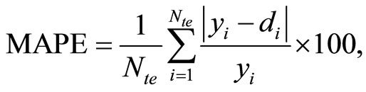 (7)
(7)
where  is the
  observed regression model output corresponding to the
  input vector
 . The Mean Absolute Error is estimated with:
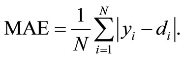 (8)
(8)
The Daily Peak MAPE consists on analyzing the MAPE in a daily fashion. That is, within the testing set  choose segments corresponding to a complete day as follows:
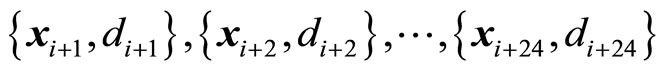
and observe the predicted daily output  then estimate the peak MAPE of that day. Formally, the DPM can be defined as follows. Let
  denote the number of days available in the testing set. Let
  be the set of sample indices corresponding to the different number of days:
where  denotes the set of indices corresponding to samples of
  day.
day.
Then the Daily Peak MAPE is obtained as follows:
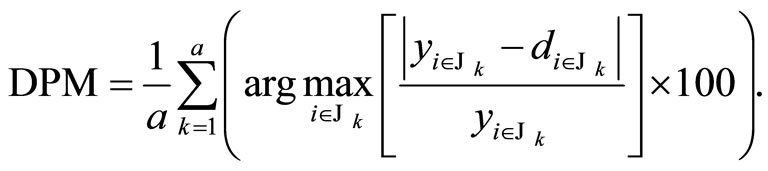 (9)
(9)
The following equation is used to compute Normalized Error:
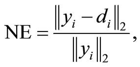 (10)
(10)
while the Root Mean Squared Error and Normalized Root Mean Squared Error are computed as follows:
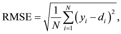 (11)
(11)
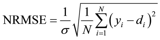 (12)
(12)
where σ is the standard deviation of y.
4.2. Quantitative Results
Table 2 shows quantitative prediction errors using the metrics explained above: MAPE, MAE, DPM, NE, RMSE, and NRMSE. According to results in Table 2the proposed LP-SVR model performs with lower error than BRT, FFNN, and LS SVM. This result is consistent for all the metrics. However, very small differences can be observed between the performance of FFNN and LP-SVR. This can be confirmed by observation in Figures 2 and 3. Figure 2 (top) shows a two-day window of

Figure 2. Two-day window of true data compared with predicted for the four different methods (top). Error residuals for the four methods (bottom).
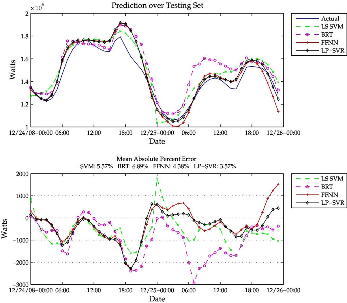
Figure 3. Christmas two-day window of true data compared with predicted for the four different methods (top). Error residuals for the four methods (bottom). Note the high prediction error between 14:00-21:00 Hr.
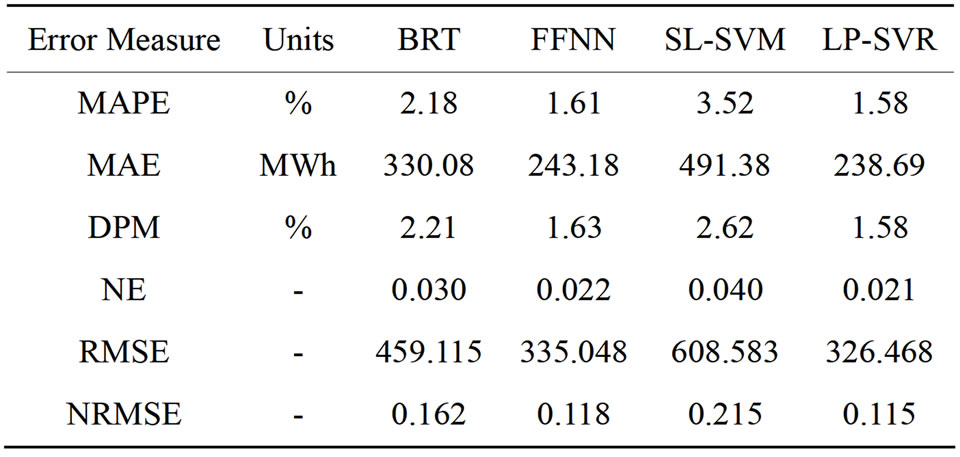
Table 2. Variables used for prediction.
true load compared with the predicted load for the four different methods, and also (bottom) shows the error residuals for the four methods.
As expected, the results of FFNN and LP-SVR exhibit very little difference. In general most methods predict the true model to a relative low error. Figure 3 shows a particular two-day window for Christmas Eve. As for many holidays, Christmas Eve is very difficult to predict due to the high variability in electricity consumption. The figure demonstrates a considerable high prediction error between 14:00-21:00 Hr on 12/24/2008.
Figure 4 shows the error distribution for the different methods. It can be concluded that FFNN and LP-SVR have smaller error variances. Similarly, Figure 5 illustrates the absolute error distribution, including the mean absolute error for each of the four methods. It can be seen that both FFNN and LP-SVR have almost the same MAEs.
An interesting analysis is the average error visualization by hour of day, shown in Figure 6. It can be seen that early morning hours (00:00-05:00) are the most “easy” to predict, i.e., can be predicted with very small error. In contrast, the late morning trough afternoon hours (06:00-22:00) are predicted with larger errors.
Figure 7 illustrates the average error by day of the week. Clearly, the days that produce higher errors are those associated with Mondays through Fridays, that represent the work week. It is important to notice the error scale between Figures 6 and 7. In Figure 6 the largest error is below 1.8 × 10⁴, while in Figure 7 the largest error is below 1.6 × 10⁴. This implies that errors are expected to be greater if the prediction is based on hourly data. From this one can conclude that the prediction is more independent of the day of the week, and more dependent on the hour of the day.
The final analysis is in regard to the statistical properties of the errors of the proposed LP-SVR model. Figures 8 through 10 shows statistical plots known as “box plots.” These plots provide the following information: on each box, the central mark is the median, the edges of the box are the 25-th and 75-th percentiles, the whiskers extend to the most extreme data points not considered outliers, and outliers (+) are plotted individually. In terms of
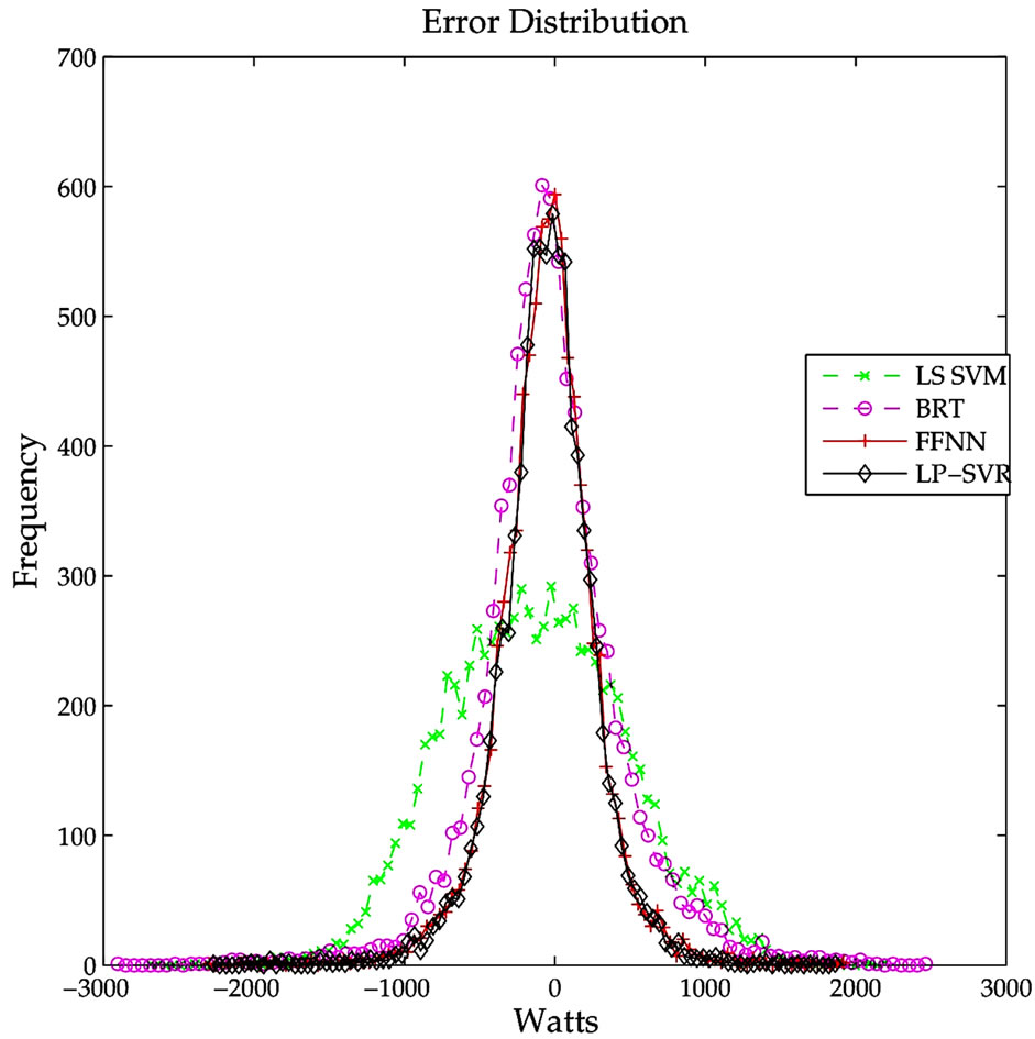
Figure 4. Error distribution for the LS SVM, BRT, FFNN, and LP-SVR regression methods. The methods with smallest variances are FFNN and LP-SVR.

Figure 5. Absolute error distribution of the LS SVM, BRT, FFNN, and LP-SVR regression methods. The vertical lines indicate the mean absolute error for each of the four methods as reported in Table 2.
error measures, it is desired that the box plots have a very small box close to zero on the error axis, the median should be close to zero, the extreme points should be close to the box, and of course no outliers are desired.
An hourly breakdown of the LP-SVR mean absolute prediction error is shown in Figure 8. It can be noticed that the early morning hours have smaller variability. Then a daily breakdown of the LP-SVR mean absolute
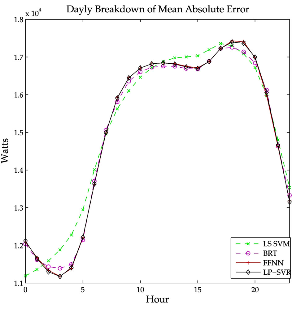
Figure 6. Average error by hour of day. Note the error proportional difference in early morning hours and afternoon hours.

Figure 7. Average error by day of week. Note the error proportional difference in working and non-working days.
prediction error appears in Figure 9, from which one can see that Mondays and Fridays have the largest average errors and that Fridays have many outliers. Finally, a monthly breakdown is shown in Figure 10. This figure clearly shows that the months of November and December exhibit the largest average errors, have the largest variability, and show many outliers.
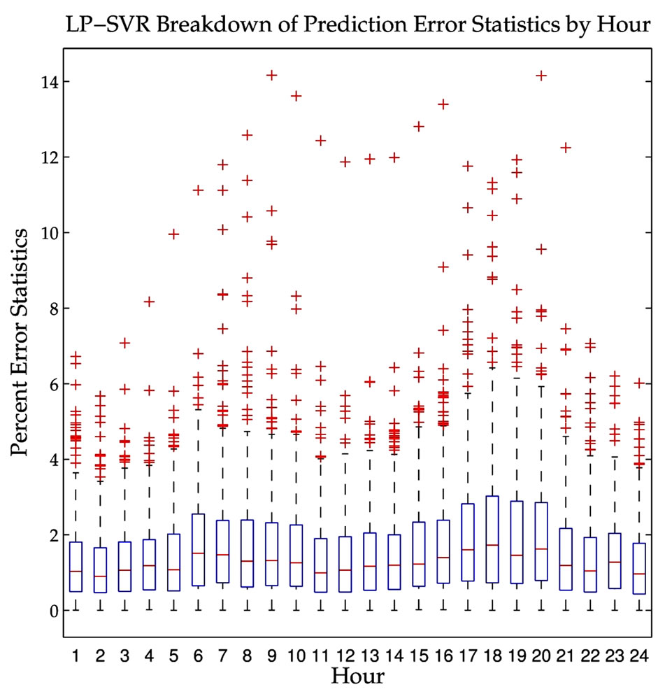
Figure 8. Hourly breakdown of the LP-SVR mean absolute prediction error. Note that the early morning hours have smaller variability.
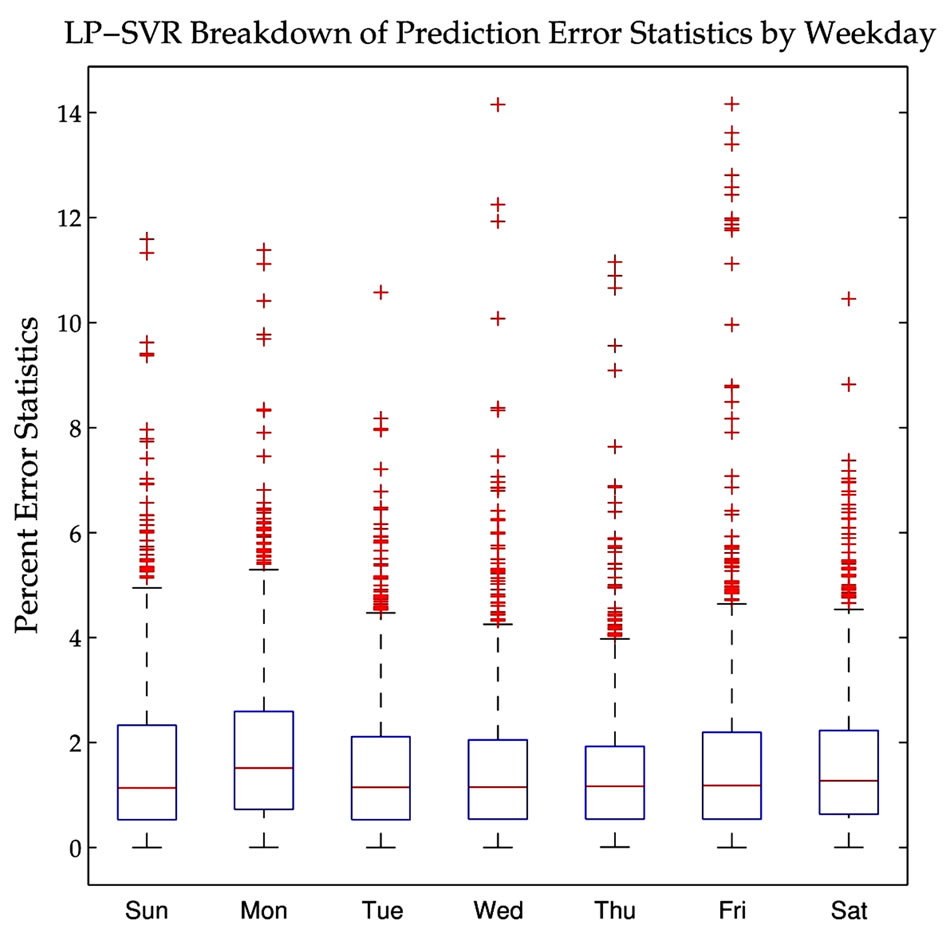
Figure 9. Daily breakdown of the LP-SVR mean absolute prediction error. Note that Mondays and Fridays have the largest average error.
5. Conclusions
This chapter presents an application of the proposed LPSVR model to electricity load prediction. A number of eight different variables are utilized to construct regression models. The study includes a comparison of the LPSVR model against other state of the art methods, such as FFNN, BRT and LS SVM.

Figure 10. Monthly breakdown of the LP-SVR mean absolute prediction error. Note that the month of December exhibits the largest average error, and the largest variability.
Experimental results indicate that the proposed LPSVR method gives the smallest error when compared against the other approaches. The LP-SVR shows a mean absolute percent error of 1.58% while the FFNN approach has a 1.61%. Similarly, the FFNN method shows a 330 MWh (Megawatts-hour) mean absolute error, whereas the LP-SVR approach gives a 238 MWh mean absolute error. This is a significant difference in terms of the extra power that would need to be produced if FFNN was used.
The proposed LP-SVR model can be utilized for predicting power loads to a very low error, and it is comparable to FFNN and over-performs other state of the art methods such as: Bagged Regression Trees, and LargeScale SVRs.
6. Acknowledgements
The author P.R.P. performed part of this work while at NASA Goddard Space Flight Center as part of the Graduate Student Summer Program (GSSP 2009) under the supervision of Dr. James C. Tilton. This work was supported in part by the National Council for Science and Technology (CONACyT), Mexico, under grant 193324/ 303732, and by the Texas Instruments Foundation Endowed Scholarship. The partial support of the SEP DGRI complementary scholarship is also acknowledged.
REFERENCES
- J. Valenzuela and M. Mazumdar, “On the Computation of the Probability Distribution of the Spot Market Price in a Deregulated Electricity Market,” 22nd IEEE Power Engineering Society International Conference on Power Industry Computer Applications, 2001. Innovative Computing for Power—Electric Energy Meets the Market, Sydney, 20 May 2001-24 May 2001, pp. 268-271.
- Y. Yuan, Y. Wu, G. Yang and W. Zheng, “Adaptive HyBrid Model for Long Term Load Prediction in Computational Grid,” 8th IEEE International Symposium on Cluster Computing and the Grid, CCGRID ’08, Lyon, 19-22 May 2008, pp. 340-347. doi:10.1109/CCGRID.2008.60
- P. Pai and W. Hong, “Support Vector Machines with Simulated Annealing Algorithms in Electricity Load Forecasting,” Energy Conversion and Management, Vol. 46, No. 17, 2005, pp. 2669-2688. doi:10.1016/j.enconman.2005.02.004
- M. Mohandes, “Support Vector Machines for Short-Term Electrical Load Forecasting,” International Journal of Energy Research, Vol. 26, No. 4, 2002, pp. 335-345. doi:10.1002/er.787
- A. Jain and B. Satish, “Clustering Based Short Term Load Forecasting Using Support Vector Machines,” PowerTech, IEEE Bucharest, Bucharest, 28 June-2 July 2009, pp. 1-8. doi:10.1109/PTC.2009.5282144
- N. E. ISO, “Nepol Zonal Load Data,” 2011. http://www.iso-ne.com
- L. Hoogerheide, J. Kaashoek and H. Dijk, “Neural NetWork Approximations to Posterior Densities: An Analytical Approach,” Econometric Institute Report, Erasmus School of Economics (ESE), Rotterdam, 2010.
- A. Gallant and H. White, “There Exists a Neural Network That Does Not Make Avoidable Mistakes,” IEEE International Conference on Neural Networks, San Diego, 24-27 July 1988, pp. 657-664. doi:10.1109/ICNN.1988.23903
- C. Bishop, “Neural Networks for Pattern Recognition,” Oxford University Press, Oxford, 1995.
- M. Canty, “Image Analysis, Classification and Change Detection in Remote Sensing: With Algorithms for ENVI/ IDL,” CRC Press, Boca Raton, 2007.
- R. Berk, “Bagging,” Statistical Learning from a Regression Perspective, Springer, New York, 2008, pp. 1-24. doi:10.1007/978-0-387-77501-2_4
- A. Cutler, D. Cutler and J. Stevens, “Tree-Based Methods,” High-Dimensional Data Analysis in Cancer Research, Springer, New York, 2009, pp. 1-19.
- R. Collobert and S. Bengio, “Svmtorch: Support Vector Machines for Large-Scale Regression Problems,” Journal of Machine Learning Research, Vol. 1, No. 2, 2001, pp. 143-160.
- E. Osuna, R. Freund and F. Girosi, “An Improved Training Algorithm for Support Vector Machines,” Proceedings of the IEEE Workshop, Neural Networks for Signal Processing, 24-26 September 1997, pp. 276-285. doi:10.1109/NNSP.1997.622408
- T. Joachims, “Making Large Scalesvm Learning Practical,” Advances in Kernel Methods—Support Vector Learning, MIT Press, Cambridge, 1999.
- P. R. Perea, “Algorithms for Training Large-Scale Linear Programming Support Vector Regression and Classification,” Ph.D. Dissertation, The University of Texas, El Paso, 2011.
- P. Rivas-Perea, J. Cota-Ruiz and J. G. Rosiles, “An Algorithm for Training a Large Scale Support Vector Machine for Regression Based Onlinear Programming and Decomposition Methods,” Pattern Recognition Letters, Vol. 34, No. 4, 2012, pp. 439-451. doi:10.1016/j.patrec.2012.10.026