Energy and Power Engineering
Vol.5 No.1(2013), Article ID:26376,8 pages DOI:10.4236/epe.2013.51003
Validation of Chaviaro Poulos and Hansen Stall Delay Model in the Case of Horizontal Axis Wind Turbine Operating in Yaw Conditions
1Department of Mechanical Engineering, Moulay Ismail University, Meknes, Morocco
2Department of Energetic, Moulay Ismail University, Meknes, Morocco
Email: Bouatem1@hotmail.com
Received November 4, 2012; revised December 11, 2012; accepted December 22, 2012
Keywords: Wind Turbine; Wake; Yaw; Stall; Stall Delay; Skewed Wake; Renewable Energy
ABSTRACT
Operating in natural wind field, the horizontal axis wind turbines are subject to cyclical variation of aerodynamic loads. This cyclical loads fluctuation is a result of two aerodynamic phenomenons: the first one is the advancing and retreating blade effect; the second one is related to the cyclical variation of induced velocity at the rotor plane. In these operating conditions, the correct prediction of this load variation is necessary to predict some important parameters linked to the fatigue and stability of free yawing turbines. The main objective of the present study is the evaluation of the azimuthal variation of normal force at different radial positions. To model the problem, the blade element momentum theory is used and wind turbine is supposed operate in yaw conditions. The aerodynamic coefficients are corrected using Chaviaropoulos and Hansen model to take into account the phenomenon of stall delay. A computer code was developed to obtain the numerical values and results are compared with measurements performed in the NASA Ames wind tunnel.
1. Introduction
Wind power is obtained by the conversion of the kinetic energy available in the wind into a useful form of energy. This category of energy is now widely seen as a serious alternative to preserve the air quality and fight against the greenhouse effect. However, improvements are still possible to make it more profitable. This can be done through a better understanding of the aerodynamic phenomena resulting from the wind interaction with the wind turbine rotor.
On the other hand, predicting the blades loads accurately is one of the most important parts of calculation in wind turbine aerodynamics. The first theory used to model the wind turbine rotor has been developed by Froude [1] and Rankine [2]. This theory considers the rotor as an instrument modifying the kinetic energy of the fluid passing through it. Froude and Rankine theory ignores the presence of the blades and the geometry of the profile.
In 1935, the blade element theory is proposed by Glauert [3]. This theory assumes that the blade can be analyzed as a number of independent elements in spanwise direction. The aerodynamic forces are calculated from aerodynamic coefficients of the profile. The integration of the aerodynamic forces along the blade provides the axial force, the torque and power of the rotor.
Afterwards, the blade element method (BE) was coupled to the momentum theory to take into account the effect of induced velocities on the rotor plane [4].
Induced velocities are calculated for each blade element by applying the theorem of the momentum in axial and tangential direction. This theory is currently improved with various adjustments taking into account the finite number of blade, blade tip losses and cyclical variation of axial induction factor in yaw conditions [4].
Wind turbines are subject to a natural environment which is always unstable. Factors such as air turbulence, the boundary layer linked to the soil and the variation of the wind speed, have a significant impact on the flow around the blades. Accordingly, the wind turbines work generally in the yaw conditions and the blades are subject to cyclical variation of the angle of attack and the aerodynamic loads.
The main aim of this study is to evaluate the azimuthal variation of normal force and induced velocity in yaw condition at different radial positions using a BEM method. The aerodynamic coefficients are corrected to take into account the phenomenon of stall delay. Results are compared with measurements made on a wind turbine in yaw condition in the NASA Ames wind tunnel.
2. Mathematical Models
2.1. BEM Theory
Classical momentum theory, introduced by Froude as a continuation of the work of Rankine, assumes that the flow is inviscid, incompressible and irrotational. In this theory the blade is divided into several elements and the study is conducted element by element. The performance of each blade element is deduced by applying the principle of momentum conservation.
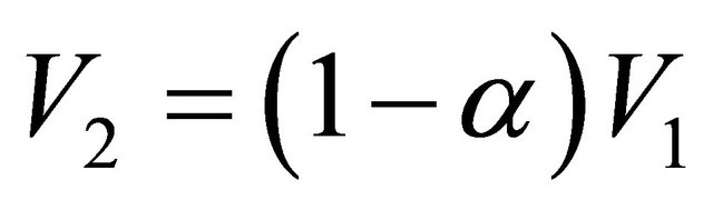
The experience shows that a wind turbine generates a wake downstream of the rotor [4,5]. This wake has a significant impact on the flow upstream. Indeed, the wind speed just before the rotor V2 (Figure 1) is slowed by the wake induced velocity. By applying the theorem of momentum in the axial direction [4,5] we obtain:
 (1)
(1)
where a is the axial induction factor.
Similar relation for rotational speed is defined with , which is called as tangential induction factor [4,5].
 (2)
(2)
where  is the tangential induced velocity at the plane just before the rotor.
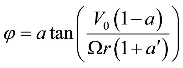
We focus here on one section of the blade located at a radius r (Figure 2). The relative wind vector denoted as W, is the resultant of an axial component  and rotational component
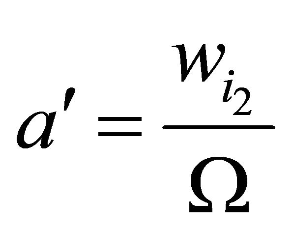
 , The rotational component is the sum of the velocity due to the blade motion r·Ω, and tangential induced velocity
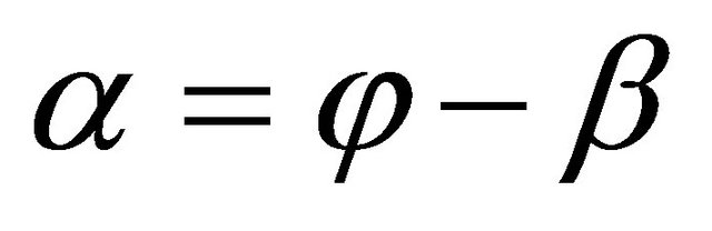
  where α is the angle of attack, β the twist angle of blade section and ϕ the angle of relative wind to the plane of rotation.
Using the conservation of linear and angular momentum equations [4,5], we obtain:
 (3)
(3)
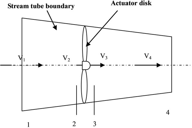
Figure 1. Actuator disk model of a wind turbine.

Figure 2. The section of a blade at radius r.
 (4)
(4)
With:
 (5)
(5)
And:
 (6)
(6)
 (7)
(7)
The aerodynamic forces applied on each blade element as shown in Figure 3 can be calculated using the aerodynamic coefficients of the profile. The element axial force (normal at the rotor plane) is given by the following equation [4,5]:
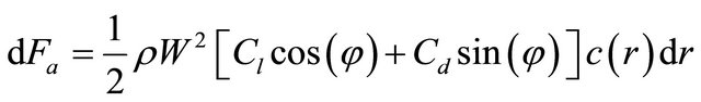 (8)
(8)
The element tangential force is given by the following equation:
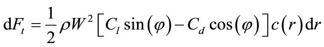 (9)
(9)
where Cl is the lift coefficient, Cd is the drag coefficient and Vrel the relative wind velocity.
2.2. Tip-Loss Model
The blade element momentum theory does not take into account the influence of vortices shed from the blade tips. These tip vortices play a major role in the induced velocity distribution at the rotor plane. To compensate for this deficiency in BEM theory, we use a correction developed by Brandt [4,5]. The Brandt correction factor F is described by the following equations:
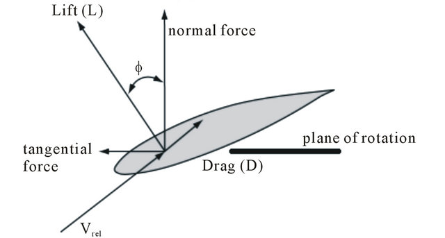
Figure 3. Forces at blade section.
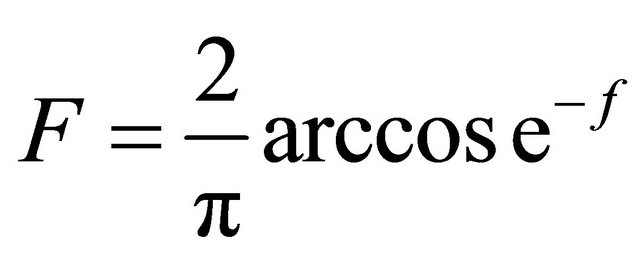 (10)
(10)
 (11)
(11)
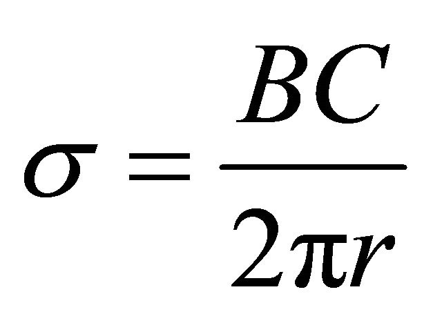
where B is the blade number, R wind turbine radius and r local radius.
The tip loss factor F is used in calculation of axial and tangential induction factor in the Equations (3) and (4), then combination of Equations (3) and (10) gives:
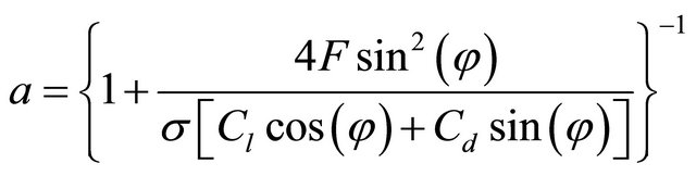 (12)
(12)
The combination of Equations (4) and (10) gives:
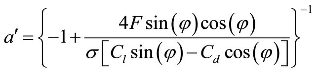 (13)
(13)
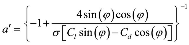
2.3. Axial Induction Factor Correction
When the axial induction factor is greater than 0.4, classical momentum theory breaks down [4,5] and the relationship (3) becomes invalid. For this operating state, Buhl developed a relationship between the axial induction factor and the thrust coefficient:
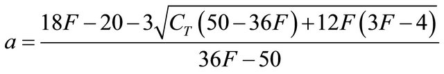 (14)
(14)
The axial induction factor is calculated for each blade element in terms of the thrust coefficient  and tip loss factor F. Then, this parameter is used to calculate the performance of wind turbine.
According to [4], the thrust coefficient CT for each blade element is calculated using the following equation:
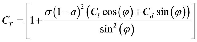 (15)
(15)
2.4. Yaw Condition
The wind turbine operates in yaw conditions when the wind direction is not perpendicular to the rotor plane.
As result, the blades are not subject to the same conditions, the blade load, the induced velocities and the angle of attack varies depending on the azimuthal position. We distinguish two main operating modes: the advancing and the retreating modes (Figure 4).
The blade will be advancing in the half plane (ANB) and retreating in half plane (BMA).
Under conditions of misalignment, the horizontal component of the wind velocity Usin(ϕy) is not null and must be taken into account in the calculation. Accordingly, the angle of attack is calculated by using the following relationship:
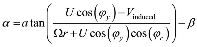 (16)
(16)
The relative wind velocity is calculated by using the following equation:
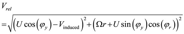 (17)
(17) 2.5. Skewed Wake Correction
In yaw conditions, the wind turbine wake is not coaxial to the rotor axis. However, the blade element momentum theory is originally developed for axisymmetric flow. The BEM model needs to be corrected to take into account this skewed wake effect. Several corrections are proposed in the literature, in this work we use the correction proposed by Pitt and Peters [4,5]:
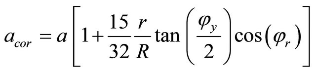 (18)
(18)
This equation is used to correct the axial induction factor initially calculated with standard models of the BEM theory.
Where acor is the corrected axial induction factor and a is the axial induction factor calculated by the method BEM.
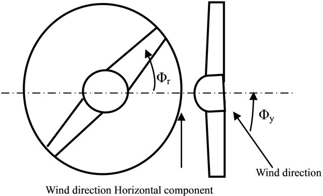
Figure 4. Advancing and retreating effect.
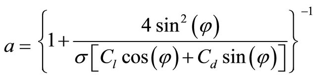
2.6. Stall Delay
At high wind velocities, a large part of the blade operates at deep stall. This phenomenon is intimately linked to the separation of the boundary layer from the surface, which can be predicted by boundary layer theory. The use of 2D aerodynamic coefficients for a rotating blade provides incorrect results. This is due to the stall delay phenomenon resulting from 3D rotational effects. Several corrections are proposed in the literature, the study carried out by [6] clearly shows that at higher wind speeds, the use of 2D airfoil data leads to an underprediction of power and thrust, while the application of the different correction models generally leads to over predictions and great disparities in the results [6].
In this work we propose the Chaviaropoulos and Hansen model because the results obtained by this model are significantly closer to the NREL data. Chaviaropoulos and Hansen model [6] correct the lift and drag coefficients to include 3D effects in the following way:
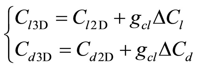 (19)
(19)
 (20)
(20)
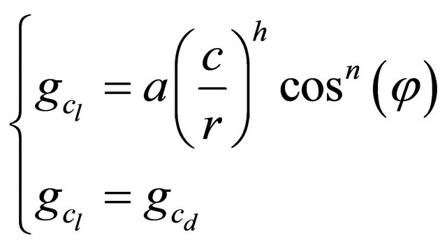
where  and
and  are functions specific to this correction model, and ΔCl and ΔCd are the difference between the Cl and Cd that would be obtained if the flow did not separate (taken here respectively as
  , and Cd = Cd (α = 0) and the Cl and Cd measured in a 2D configuration.
Referring to the work done by [6], the constants take the following values: a = 2.2, h = 1 and n = 4.
3. Computational Algorithm
The objective is to evaluate the normal force applied to each blade element. The calculation is performed for different azimuthal positions.
The solution cannot be found directly because of the nonlinear nature of the equations system. For each element along the span of the blade, the iteration procedure starts with an estimation of factors a and a׳. These two factors are used to determine the flow angle on the blade using Equation (16). Then the blade section properties are used to estimate the thrust coefficient with the Equation (15). Afterword the factors a is calculated. The Equation (14) is used when a is greater than 0.4 and if a is lower than 0.4, we use the Equation (12).
In the flowing step, the factor a׳ is calculated with the Equation (13). Finally the effect of skewed is included using the Equation (18). This process is repeated until the convergence of the axial induction factor a. The normal force is calculated after convergence. The stall delay effect is taken into account in the determination of Cl and Cd.
The main steps of the simulation code are presented in the algorithm shown in Figure 5.
4. Validation of the Algorithm
Validation of the algorithm requires a comparison of calculations results with experiment. In the present work, we refer to wind tunnel tests from the National Renewable Energy Laboratories. These tests were performed in the year 2000, in the biggest wind tunnel in the world (24.4 × 36.6 m), on a wind turbine with the following characteristics [7]:
• The rotor diameter is 10 m;
• The turbine is two-bladed;
• The blade have a linear taper with a maximum chord of 0.737 m at 25% span and 0.356 m at 100% span;
• The blade have a non-linear twist of 22.5 degrees over the blade;
• The airfoil is the S809 airfoil, over entire span;
• The turbine has an asynchronous generator with a rated rotor speed of 72 rpm.
One of the blades is equipped at 5 radial positions with 22 pressure taps each. The measurement sections are located at 0.3R, 0.47R, 0.63R, 0.80R and 0.95R [7].
NREL performed measurements for a wide variety of conditions namely tunnel speeds, pitch angles and yaw angles. In the present study we compare our results with measurements made with a yaw angle of 30 degrees and pitch angle of 0 degree. In the different calculations the structure is assumed to be rigid, mass induced loads are neglected and the wind speed is constant and homogenous.
Calculations are performed for three tunnel speeds: 5 m/s, 10 m/s and 15 m/s at 30% and 95% span.
Figures 6 and 7 represent the evolution of normal force as a function of the azimuth angle at 30% and 95% of the blade. Measured and calculated curves show the same tendencies and are almost in phase.
Generally speaking, for an air speed of 5 m/s, the calculated curves show the same tendencies as the measured curves. The agreement between calculated and measured curves is excellent in terms of shape. However, a small difference in amplitude is observed.
Figures 8 and 9 show the normal force at 30% and 95% span for an air speed equal to 10 m/s. We observe once again that the calculated and measured curves have the same tendencies with a slight difference in amplitude.
We conclude that the proposed algorithm gives satisfactory results for this tranche of speed at the different radial positions.
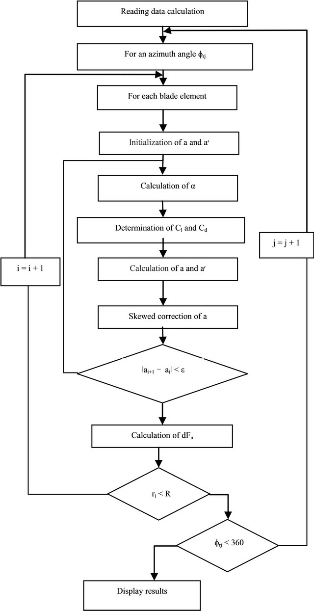
Figure 5. Computational algorithm.
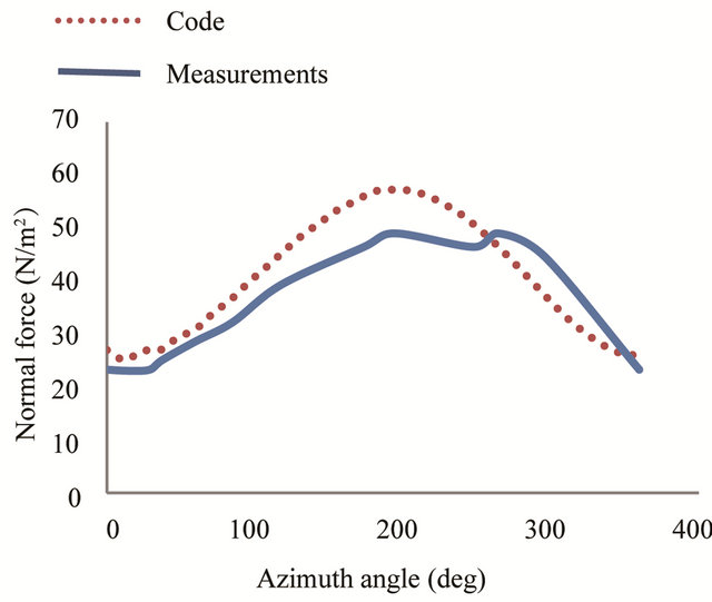
Figure 6. Normal force distribution at 30% span, for wind speed of 5 m/s.
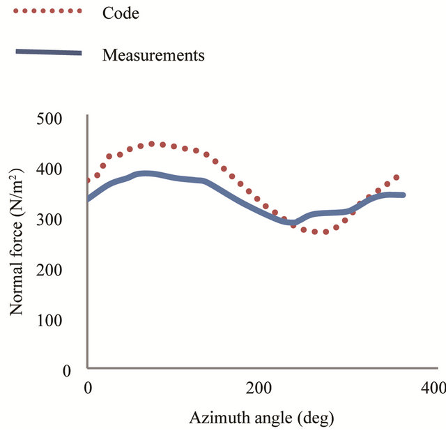
Figure 7. Normal force distribution at 95% span, for wind speed of 5 m/s.
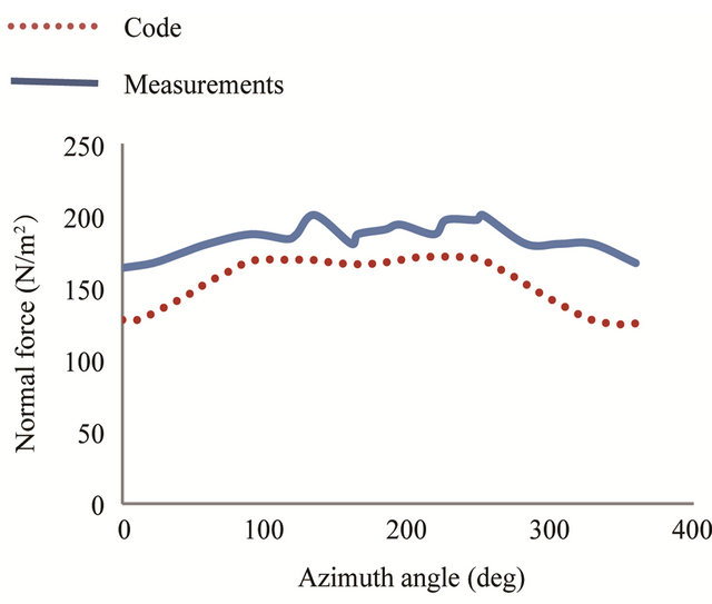
Figure 8. Normal force distribution at 30% span, for wind speed of 10 m/s.
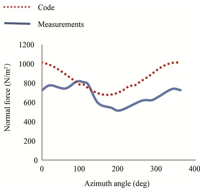
Figure 9. Normal force distribution at 95% span, for wind speed of 10 m/s.
The same comparison is performed for an air velocity of 15 m/s. Figures 10 and 11 show the normal force at 30% and 95% span. At these high tunnel speeds, the curves are almost in phase and have similar tendencies. Differences are found in the amplitude.
5. Results Analysis
The cyclic variation of the normal force is strictly related to the distribution of the relative velocity at the rotor plane and angle of attack. These two parameters are given by Equations (17) and (18) which show clearly that the azimuthal variation of the normal force can be a result from:
• The variation of angle of attack caused by the advancing and retreating blade effect;
• The variation of the relative velocity caused by advancing and retreating blade effect;
• The variation of angle of attack caused by the cyclical variation of induced velocity;
• The variation of the relative velocity caused by the cyclical variation of induced velocity.
The study of the impact of the angle of attack on the normal force requires the examination of the distribution of this parameter at rotor plane.
The Figure 12 shows the evolution of the angle of attack as a function of the azimuthal position at 30% span for a wind speed of 5 m/s.
We note that the variation of angle of attack is reflected into the variation of normal force Figure 6. Indeed, the distribution of the normal force and the angle of attack are in good correlation in terms of shape.
The Figure 13 shows the evolution of the angle of attack as a function of the azimuthal position at 95% span for a wind speed of 5 m/s.
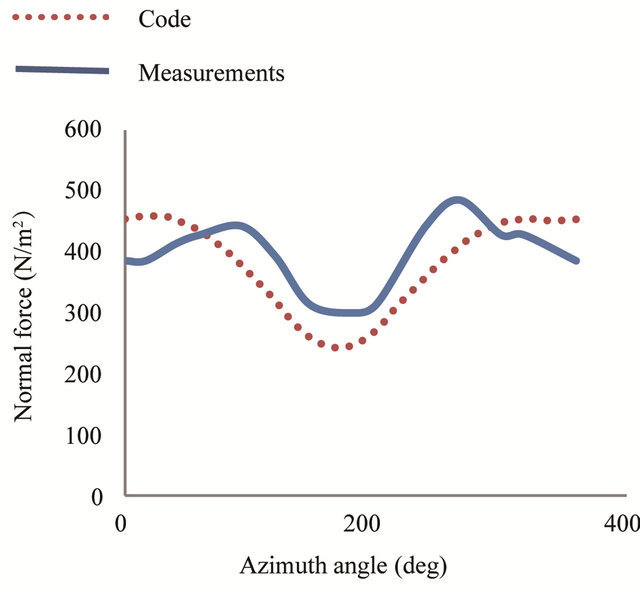
Figure 10. Normal force distribution at 30% span, for wind speed of 15 m/s.
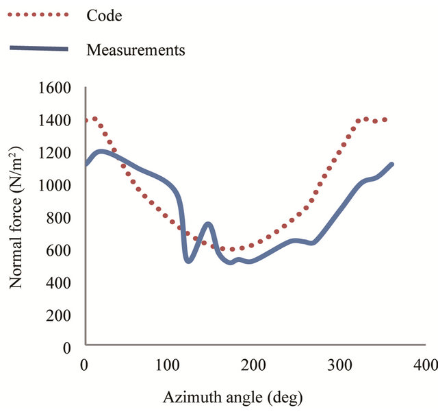
Figure 11. Normal force distribution at 95% span, for wind speed of 15 m/s.
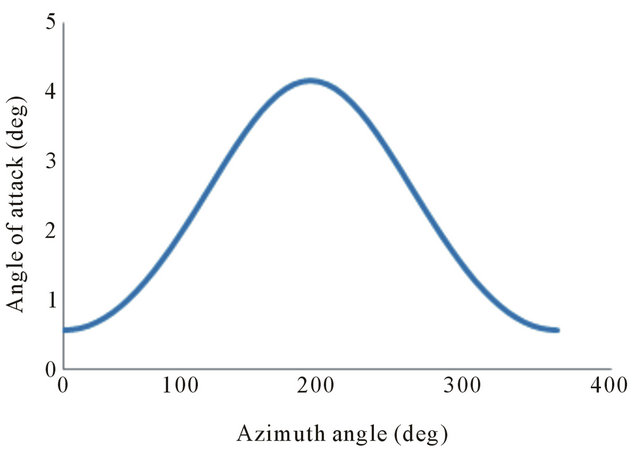
Figure 12. Angle of attack distribution at 30% span, for wind speed of 5 m/s.
The examination of the curve represented in Figure 7 and the curve represented in Figure 13 clearly shows that the azimuthal variation of the normal force is a result of the azimuthal variation of the angle of attack. The two curves are in phase and have the same tendencies.
The Figure 14 shows the evolution of the angle of attack as a function of the azimuthal angle at 30% span for a wind speed of 15 m/s.
The Figure 15 shows the evolution of the angle of attack as a function of the azimuthal angle at 95% span for a wind speed of 15 m/s.
We note that the curves representing the variation of the angle of attack, Figures 14 and 15 are opposed to the normal force curves, Figures 10 and 11. This result can be explained by the stall effect. Indeed, when the angle of attack exceeds the stall angle, the increase of this parameter lead to a drop in performance of the rotor, especially the normal force.
6. Conclusions
This work focuses on the application of the BEM method
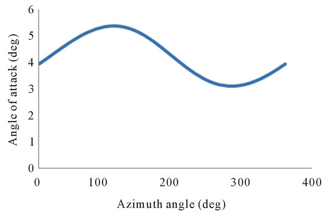
Figure 13. Angle of attack distribution at 95% span, for wind speed of 5 m/s.
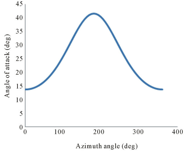
Figure 14. Angle of attack distribution at 30% span, for wind speed of 15 m/s.
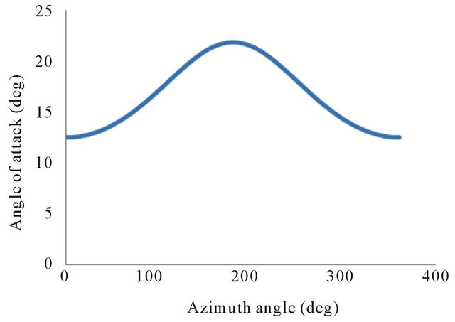
Figure 15. Angle of attack distribution at 95% span, for wind speed of 15 m/s.
for the study of wind turbine aerodynamic behavior in yaw condition.
Based on this theory we have developed a FORTRAN code which allows the calculation of the main aerodynamic parameters of the wind turbine. We particularly interested in the variation of the normal force at a given section of the blade as a function of the azimuthal angle.
For the validation of the numerical code, we have compared our results with the experimental data of NASA Ames. This comparison demonstrates the ability of the used model to produce results consistent with experience with an acceptable tolerance. However, we have demonstrated the existence of a difference in amplitude due to the different assumptions adopted in this model.
This study show that the variation of the normal force as a function of the azimuthal angle is periodic. This fluctuation is due to the skewed wake and the advancing and retreating effect. On the other hand, the study confirms that the skewed wake effect plays a major role in the aerodynamic loads calculation at lower wind speed. However, the advancing and retreating blade effect is important at high wind speed and it can provide a strong dynamic stall effect. This phenomenon explains the important difference between experiment and theory at higher wind speed.
REFERENCES
- R. E. Froude, “On the Part Played in Propulsion by Difference in Pressure,” Transactions of the Institution of Naval Architects, 1889, pp. 390-423.
- W. J. M. Rankine, “On the Mechanical Principles of the Action of Propellers,” Transactions of the Institution of Naval Architects, 1865, pp. 13-39.
- H. Glauert, “Airplane Propellers,” In: W. F. Durand, Ed., Aerodynamic Theory, Vol. 4, 1934, p. 332.
- P. J. Moriartry and A. C. Hansen, “Aerodyn Theory Manual,” National Renewable Energy Laboratory, 2005, NREL TP-500-36881.
- J. Hernandez and A. Crespo, “Aerodynamics Calculation of the Performance of Horizontal Axis Wind Turbines and Comparison with Experimental Results,” Wind Engineering, Vol. 11, No. 4, 1987, pp. 177-187.
- S. P. Breton, “Study of the Stall Delay Phenomenon and of Wind Turbine Blade Dynamics Using Numerical Approaches and NREL’s Wind Tunnel Tests,” Doctoral Thesis, Norwegian University of Science and Technology, Trondheim, 2008.
- J. G. Shepers, “Final Report of IEA Annex XX: Comparison between Calculations and Measurements on a Wind Turbine in Yaw in the NASA-Ames Wind Tunnel,” ECN-E-07-072.