Communications and Network
Vol.07 No.01(2015), Article ID:53719,8 pages
10.4236/cn.2015.71003
Improving Queuing System Throughput Using Distributed Mean Value Analysis to Control Network Congestion
Faisal Shahzad1, Muhammad Faheem Mushtaq1, Saleem Ullah1*, M. Abubakar Siddique2, Shahzada Khurram1, Najia Saher1
1Department of Computer Science & IT, The Islamia University of Bahawalpur, Bahawalpur, Pakistan
2College of Computer Science, Chongqing University, Chongqing, China
Email: faisalsd@gmail.com, faheem.mushtaq88@gmail.com, *saleemullah@iub.edu.pk, abubakar.ahmadani@gmail.com, khurram@iub.edu.pk, najia@iub.edu.pk
Copyright © 2015 by authors and Scientific Research Publishing Inc.
This work is licensed under the Creative Commons Attribution International License (CC BY).
http://creativecommons.org/licenses/by/4.0/


Received 12 June 2014; accepted 30 January 2015; published 2 February 2015
ABSTRACT
In this paper, we have used the distributed mean value analysis (DMVA) technique with the help of random observe property (ROP) and palm probabilities to improve the network queuing system throughput. In such networks, where finding the complete communication path from source to destination, especially when these nodes are not in the same region while sending data between two nodes. So, an algorithm is developed for single and multi-server centers which give more interesting and successful results. The network is designed by a closed queuing network model and we will use mean value analysis to determine the network throughput (b) for its different values. For certain chosen values of parameters involved in this model, we found that the maximum network throughput for
 remains consistent in a single server case, while in multi-server case for
 throughput surpass the Marko chain queuing system.
Keywords:
Network Congestion, Throughput, Queuing System, Distributed Mean Value Analysis

1. Introduction
Networks where a communication path between nodes doesn’t exist refer to delay tolerant networks [1] [2] ; they communicate either by already defined routes or through other nodes. Problem arises when network is distributed and portioned in to several areas due to the high mobility or when the network extends over long distances and low density nodes. The traditional approach [3] for the queuing system was to design a system of balance equations for the joint property of distributed vector value state. The traditional approaches to the system of Markovian [4] queuing systems were to formulate a system of algebraic equations for the joint probability distributed system vector valued state, which was the key step introduced by Jackson [5] , that for a certain types of networks the solutions of the balance equation is in the form of simple product terms. All remained to be normalized numerically to form the proper probability distribution In case of networks with congested routing chains, this normalization turned out to be limited and degrades the system efficiency as well.
Therefore, in practical these distribution contains an extra detail, such as mean queue size, mean waiting time and throughput is needed. The framework of conventional algorithm shows that these properties can be obtained by normalizing constants. The proposed algorithm given in this paper correlates directly with the required statistics. Its complexity is asymptotically is almost equal to the already defined algorithms, but the implementation of program is very simple.
Choosing the right queuing discipline and the adequate queue length (how long a packet resides in a queue) may be a difficult task, especially if your network is a unique one with different traffic patterns. Monitoring of the network determines which queuing discipline is adequate for the network. It is also important to select a queuing length that is suitable for your environment. Configuring a queue length that is too shallow could easily transmit traffic into the network too fast for the network to accept, which could result in discarded packets. If the queue length is too long, you could introduce an unacceptable amount of latency and Round-Trip Time (RTT) jitter. Program sessions would not work and end-to-end transport protocols (TCP) would time out or not work.
Because queue management is one of the fundamental techniques in differentiating traffic and supporting QoS functionality, choosing the correct implementation can contribute to your network operating optimally.
2. Mean Value Evaluation
Included in the Quality of Service Internetwork architecture is a discipline sometimes called queue management. Queuing is a technique used in internetwork devices such as routers or switches during periods of congestion. Packets are held in the queues for subsequent processing. After being processed by the router, the packets are then sent to their destination based on priority.
In the queuing network, the traditional approach to find the solution is using characteristics of a continuous time markov chain to formulate a system of balance equation for the joint probability distribution of the system state. The solution of the balance equations, for certain classes of networks such as Jackson networks and Gordon-Newell networks is in the form of a product of simple terms, see [6] . In general, the joint probability is not so simple and sometime it is inefficient to pursue. If we only interested in the average performance measure such as average waiting time, average response time or network throughput, we do not need the steady-state probabilities of the queue length distributions. In this stage, we will use an approach so called mean value analysis. The algorithm for this approach works directly to the desired statistics and has been developed and applied to the analysis of queuing networks, for example see [7] . The mean value analysis is based on the probability distribution of a job at the moment it switches from one queue at a server to another and the steady state probability distribution of jobs with one job less. This relation is known as arrival theorem for closed queuing networks. In a closed queuing network, the bottleneck is the queue with the highest service demand per passage.
Using the arrival theorem, if a job move from queue i to queue j in a closed queuing networks with K jobs in it, will find on average
 jobs. With this result and assuming that a job is served in a first come first served basis, a relation between the average performance measure in this network with K jobs and
 job can be performed recursively.
3. Proposed Mechanism
Mean value analysis depends on the mean queue size and mean waiting time. This equation applied to each routing chain and separately to each service center will furnish the set of equations which will easily solved numerically. The proposed algorithm is simple and avoid overflow, underflow actions which may arise with traditional algorithms. All mean values in the algorithm are calculated in a parallel manner. Thus memory requirement is higher than the previous ones, but new mechanism is relatively faster in multi-server scenarios.
We have considered the closed multi-chain queuing system which has the product form solution. Suppose C is a routing chain and S is a service center. Each chain contains a fixed number of customers who processed through subset of services using Markov chain technique, while service providers adopt one of the following mechanisms.
1) FIFO: customers are serviced in order of arrival, and multi-servers can be used.
2) Priority Queuing: customers are serviced according to the traffic categorization.
3) WFQ (Weighted Fair Queuing): gives low-volume traffic flows preferential treatment and allows higher-volume traffic flows to obtain equity in the remaining amount of queuing capacity. WFQ tries to sort and interleave traffic by flow and then queues the traffic according to the volume of traffic in the flow.
4) PS: Customers are served in parallel by a single server.
5) LCFSPR: customers are served in reverse order of arrival by a single server, (Last come first served preemptive resume).
Now we assume that all the servers have constant service rate using multiple FCFS service centers starting with the following consequences, which relates mean waiting time
 to the mean queue size of the system
 with one customer less in the chain r making the following equation,
 (1)
(1)
 is the equilibrium mean waiting time of chain
 at service center

 is the mean value of the service demand,
 represent equilibrium mean queue size,
 is size of chain
 , and
, and
 is the R-dimensional unit vector. From the definition it is clear that
 (2)
(2)
 is the average number of customers in chain between successive visits, then the mean number of visits
 and its waiting time per visit with service center visited by chain
 is described as
 (3)
(3)
where
 is the throughput of chain
 , considering service center
 i.e.
i.e.
 then for multiple service stations each one yields the following relation,
 (4)
(4)
The above equations applicable for recursive analysis of mean queuing size, meat waiting time and system throughput. The initial point can be set as,
 For all
 and
and .
.
To make the substitution in an algorithmic form, we have
 and
and

3.1. Mathematical Model
Our model is defined on a one-dimensional closed system consisting of M cells i.e. Figure 1. A closed queuing network model is justified for steady state conditions. In steady state, for a single-entry and single-exit lane, the traffic flow into the system will be equal to the traffic flow out of the system. We approximate this as a closed system where the number of vehicles remains the same. Each cell can either be empty or occupied by one vehicle. To start with, we assume vehicles of identical size. Since the system is closed, the number of vehicles remains constant, say equal to . Thus the system density can be defined as
 . Hereon, this model will be referred to as the Path Cell Network model. A vehicle moves from the first to the second and so on to the
 cell and then back to the first cell. It is apparent that the system has attributes of a queuing system with FIFO discipline. In the past, the general modeling of traffic using Queuing Theory has been macroscopic, but here instead of treating the whole closed link as a single queue, we consider it as a network of queues. The Path Cell Network model at first appears to be a cumbersome one as each cell has limited space and, therefore, each queue in the network limited buffer space. But, our task can be made much easier by our definition of the servers. The exact working of the model is as follows:
Being a single lane model each vehicle moves to the next cell if empty or waits, and then moves when the vehicle ahead vacates the cell. Thus there can only be two configurations for a particular vehicle: either the cell
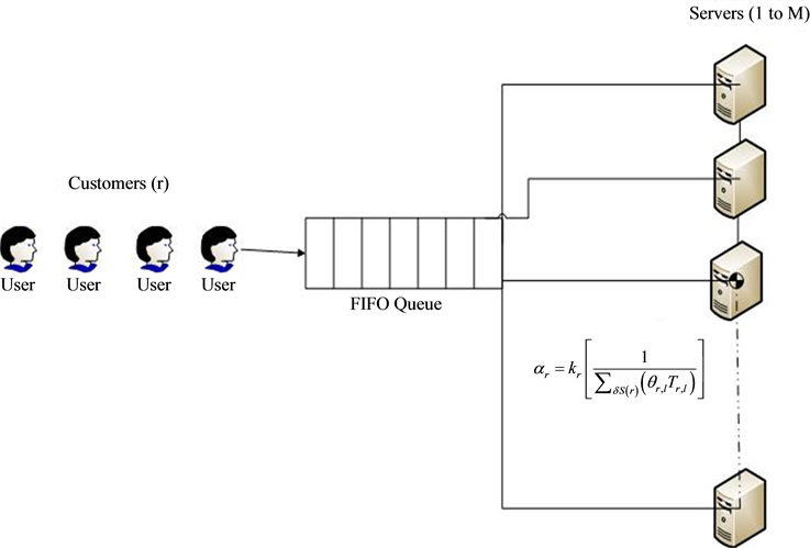
Figure 1. Queuing model.
ahead is empty or occupied. We say a vehicle is in service when the cell ahead is empty and “waiting” if it is occupied.

In effect, each empty cell acts as a server, and at any point in time there are always
 servers in the system that keeps changing their positions. These dynamic cells act as servers to
 queues in the system that together form a closed network. The number of waiting units in each queue can be counted as the total number of vehicles between the empty cell and the one empty behind it. Thus if there are two consecutive empty cells, both act as servers with one of them having zero queue size. Service in each queue is assumed to be exponential, and for the basic Path Cell Network model, assuming identical vehicles, the service rate of each vehicle is also taken to be the same. As the service is exponential, from the Poisson-in-Poisson-out property inter-arrival times at each queue are also exponential.
The model we claim can be mapped onto a cyclic Jackson network with
 cells and N customers. Thus, effectively, a path segment with very limited buffer space at each queue is mapped onto a well-known cyclic queuing network with buffer space of size N.
The results of a cyclic Jackson network are well known. A state is indicated by

and
 indicates the number of units at each stage of the closed queuing network. The probability of being in a state
 is written as
 Transitions between states occur when a unit enters or leaves a stage. Service rate
 at each stage is allowed to be dependent upon the number of units
 in the stage. Then
 (5)
(5)
while,

In this case we have consider the service rate and probability at each node and stage is same and equal to the inverse of the number of ways of selecting
 out of
 places as customers and remaining
 places being the partitions, it is calculated as
 ,
,
here throughput
 of the network can be calculated as
 (6)
(6)
where
 is simply the number of ways of selecting
 out of the last
 places as customers, the first place being a partition
 (7)
(7)
For the corresponding network number of queues , throughput
 of the network is obtained by scaling
 using the following relation
 (8)
(8)
After scaling, throughput becomes
 (9)
(9)
For ,
,

The algorithm starts with an empty network (zero customers), then increases the number of customers by 1 until it reaches the desired number of customers of chain .
.
The average waiting time in this closed queuing network and the average response time per visit are given by the following formulas:
 (10)
(10)
where,
 is the service time, and
 is waiting time. To obtain the average response time per passage, the above equation can be obtained by each time visit ratio as
 (11)
(11)
where,
 is response time and
 is each time visit. The expected number of jobs in queue
 is given by little’s formula [6] as.
 (12)
(12)
3.2. Case Studies
Now we have to implement our model in single and multi-server scenarios to calculate throughput and mean waiting time.
a) SINGLE SERVER CASE
Initialize
 for all

 ,
, , and
, and
If at the service centers customers are delayed independently
 of other customers, then we have the following steps,
 (13)
(13)
Then we have a little’s equation for chains and service centers as,
 (14)
(14)
 (15)
(15)
The operations count for this algorithm is bounded by
 additions and
 multiplication/ divisions. This is the same as the convolution algorithm in its most efficient. However, Algorithm 1 completely avoids a genuine problem of the convolution algorithm, namely, that the floating point range of many computers may be easily exceeded. Scaling, as discussed in [8] , may partially alleviate the problem. Yet the scaling algorithm is complex and does not always work. The authors have seen several well-posed modeling problems involving relatively large populations (e.g., >100) and type D service centers which were not solvable in the range of floating point numbers 1E ± 75, despite scaling. The storage requirement is of the order
 as compared to
 for the convolution algorithm.
We now proceed to extend the computational procedure to handle FCFS service centers with multiple constant unit rate servers. The mean value Equation (14) for such a center can be written as
 (16)
(16)
where
 is the mean service demand, which is assumed to be independent of the chain. The calculation is complicated by the marginal queue size probabilities, which we have to carry along in the recursive scheme. This can be done by means of Lemma 1, which allows calculation of
 ,
,
 from previously computed values. In order to keep the recursion going, we need an independent equation for
 , which is obtained from the following relations
 (17)
(17)
where
 (18)
(18)
From Equations (17) & (18) we can have the mean number of idle servers as , which is just like a little’s equation implemented to the set of servers.
b) MULTISERVER CASE
Step 1: Parameters Initialization

Step 2: Main Loop, same as in single server case.
Step 3: Additional Corollary for Multi-servers.
 (19)
(19)
For
 and each FCFS multi server center
 , while for other service centers use the equation of step 3 in single server case.
Step 4: Little’s equation for chains having , same as in single server case.
Step 5: Little’s equation for service centers having , same as in single server case.
Step 6: Additional step for calculating marginal queue size under main loop for each multi FCFS service center
 and
and .
.
 (20)
(20)
 (21)
(21)
 (22)
(22)
The process evaluate per multi service center and per recursive step of the order
 additions and
 multiplications. We observe that it grows linearly with M.
c) Queuing Theory Limitations
The assumptions of classical queuing theory may be too restrictive to be able to model real-world situations exactly. The complexity of production lines with product-specific characteristics cannot be handled with those models. Therefore specialized tools have been developed to simulate, analyze, visualize and optimize time dynamic queuing line behavior.
For example; the mathematical models often assume infinite numbers of customers, infinite queue capacity, or no bounds on inter-arrival or service times, when it is quite apparent that these bounds must exist in reality. Often, although the bounds do exist, they can be safely ignored because the differences between the real-world and theory is not statistically significant, as the probability that such boundary situations might occur is remote compared to the expected normal situation. Furthermore, several studies [9] [10] show the robustness of queuing models outside their assumptions. In other cases the theoretical solution may either prove intractable or insufficiently informative to be useful.
Alternative means of analysis have thus been devised in order to provide some insight into problems that do not fall under the scope of queuing theory, although they are often scenario-specific because they generally consist of computer simulations or analysis of experimental data.
4. Simulation Results & Discussion
The network bottleneck is the fast server. For
 the fast server is also the network bottleneck, but when
 , the network bottleneck is the slow server.
The determination of network throughput for different values of β is calculated recursively. Every job arrives at server serve immediately (FCFS). Figure 2 shows the plot between β and network throughput and clearly shows the difference between two schemes with consistence behavior.
Figure 3 describes value by value
 performance with rival scheme. Markov Chain scheme started very confidently achieving 35 Mbps at
 but later at
 our proposed scheme performance increases in terms of Mbps which remain consistent. So in multi-server case for every value of
 the queuing systems performs well. After deep analysis on other resulted files created after simulation, we have seen that size of packet is also increases as throughput increase which also help in improving system overall performance.
Figure 4 shows queuing system mean waiting time which increases as usual as the number of customer in chain increases. But still our proposed model is somehow better while comparing with other.
This means waiting time also one of the main objectives of my future work. To define and construct a model in which mean waiting system decreases as the number of customers increases by implementing some grid

Figure 2. Throughput and consistency behavior between two schemes .
.

Figure 3. Throughput and consistency behavior (Multi-Server Scenario).

Figure 4. Queuing mean waiting time.
computing functionalities. Also developing a queuing network model for multi-hop wireless ad hoc networks keeping same objectives, used diffusion approximation to evaluate average delay and maximum achievable per-node throughput. Extend analysis to many to one case, taking deterministic routing into account.
Acknowledgements
This research work was partially supported by NSF of china Grant No. 61003247. The authors also would like to thanks the anonymous reviewers and the editors for insightful comments and suggestions.
Cite this paper
FaisalShahzad,Muhammad FaheemMushtaq,SaleemUllah,M. AbubakarSiddique,ShahzadaKhurram,NajiaSaher, (2015) Improving Queuing System Throughput Using Distributed Mean Value Analysis to Control Network Congestion. Communications and Network,07,21-29. doi: 10.4236/cn.2015.71003
References
- 1. Jones, E.P.C., Li, L. and Ward, P.A.S. (2005) Practical Routing in Delay-Tolerant Networks. Proceedings of ACM SIGCOMM Workshop on Delay Tolerant Networking (WDTN), New York, 1-7.
- 2. Zhao, W., Ammar, M. and Zegura, E. (2005) Controlling the Mobility of Multiple Data Transport Ferries in a Delay-Tolerant Network. INFOCOM, 1407-1418.
- 3. Bambos, N. and Michalidis, G. (2005) Queueing Networks of Random Link Topology: Stationary Dynamics of Maximal Throughput Schedules. Queueing Systems, 50, 5-52.
http://dx.doi.org/10.1007/s11134-005-0858-x - 4. Kawanishi, K. (2005) On the Counting Process for a Class of Markovian Arrival Processes with an Application to a Queueing System. Queueing Systems, 49, 93-122.
http://dx.doi.org/10.1007/s11134-005-6478-7 - 5. Masuyama, H. and Takine, T. (2002) Analysis of an Infinite-Server Queue with Batch Markovian Arrival Streams. Queueing Systems, 42, 269-296. http://dx.doi.org/10.1023/A:1020575915095
- 6. Armero, C. and Conesa, D. (2000) Prediction in Markovian Bulk Arrival Queues. Queueing Systems, 34, 327-335. http://dx.doi.org/10.1023/A:1019121506451
- 7. Bertsimas, D. and Mourtzinou, G. (1997) Multicalss Queueing System in Heavy Traffic: An Asymptotic Approach Based on Distributional and Conversational Laws. Operations Research, 45, 470-487.
http://dx.doi.org/10.1287/opre.45.3.470 - 8. Reiser, M. (1977) Numerical Methods in Separable Queuing Networks. Studies in Management SCI, 7, 113-142.
- 9. Chandy, K.M., Howard, J., Keller, T.W. and Towsley, D.J. (1973) Local Balance, Robustness, Poisson Departures and the Product Forms in Queueing Networks. Research Notes from Computer Science Department, University of Texas at Austin, Austin.
- 10. Knadler Jr., C.E. (1991) The Robustness of Separable Queueing Network Models. In: Nelson, B.L., David Kelton, W. and Clark, G.M., Eds., Proceedings of the 1991 Winter Simulation Conference, 661-665.
NOTES

*Corresponding author.