Communications and Network
Vol. 4 No. 1 (2012) , Article ID: 17492 , 12 pages DOI:10.4236/cn.2012.41003
L(0,1)-Labelling of Cactus Graphs
1Department of Applied Mathematics with Oceanology and Computer Programming, Vidyasagar University, Midnapore, India
2Department of Mathematics, National Institute of Technology, Durgapur, India
Email: {mmpalvu, afsaruddinnkhan, anita.buie}@gmail.com
Received August 9, 2011; revised October 14, 2011; accepted November 1, 2011
Keywords: Graph labelling; code assignment; L(0,1)-labelling; cactus graph
ABSTRACT
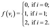
An  -labelling of a graph
  is an assignment of nonnegative integers to the vertices of
  such that the difference between the labels assigned to any two adjacent vertices is at least zero and the difference between the labels assigned to any two vertices which are at distance two is at least one. The span of an
  -labelling is the maximum label number assigned to any vertex of
 . The
. The  -labelling number of a graph
 , denoted by
  is the least integer
  such that
  has an
  -labelling of span
 . This labelling has an application to a computer code assignment problem. The task is to assign integer control codes to a network of computer stations with distance restrictions. A cactus graph is a connected graph in which every block is either an edge or a cycle. In this paper, we label the vertices of a cactus graph by
  -labelling and have shown that,
  for a cactus graph, where
  is the degree of the graph
 .
.
1. Introduction
Cactus graph is a connected graph in which every block is a cycle or an edge, in other words, no edge belongs to more than one cycle. Cactus graphs have been extensively studied and used as models for many real-world problems. This graph is one of the most useful discrete mathematical structures for modelling problems arising in the real-world. It has many applications in various fields, like computer scheduling, radio communication system, etc. Cactus graphs have been studied from both theoretical and algorithmic points of view. This graph is a subclass of planar graph and superclass of tree.
An  -labelling of a graph
  is a function of
  from its vertex set
  to the set of nonnegative integers such that
  if
if  and
and  if
if , where
  is the distance between the vertices
  and
and , i.e., the number of edges between
  and
and . The span of an
  -labelling
  of
of  is max
 . The
. The  -labelling
  of
of  is the smallest
  such that
  has a
has a  - labelling of span
 .
.
An interesting graph-labelling problem comes from the radio frequency assignment problem, as well as code assignment in computer networks. One version of the radio channel assignment problem [1] is to assign integer channels to a network of transmitters with distance restrictions, such that the several labels of interference between nearby transmitters are avoided and the span of the label used is minimized. A variation of the problem is code assignment in computer networks, i.e., to assign integer control codes to a network of computer stations with distance restrictions.
Bertossi and Bonuccelli [2] introduced a kind of code assignment to avoid hidden terminal interference; this is as follows. Since some modern computer networks consist of including mobile computers or computer displaced in wide areas, they need to use broadcast communication media such as busses (only in local area networks) or radio frequencies. The computer network which communicates by radio frequencies is called Packet Radio Network. It consists of computer stations (computers and transceivers), in which the transceivers broadcast outgoing message packets and listen for incoming message packets. Unconstrained transmission in broadcast media may lead to collision on interference, i.e., there is the time-overlap of two or more incoming message packets received at the destination station. This results in damaged useless packets at the destination. Collided message packets must be retransmitted. That increases the time delay of the transmission, and hence lowers the system throughput. Several protocols have been devised to reduce or eliminate the collisions. They form the medium access control sublayer. For example, under Code Division Multiple Access protocol, the collision-free property is guaranteed by the use of proper assignment of orthogonal control codes to stations and the spread of spectrum communication techniques (e.g., hopping over different time slots or frequency bands).
We represent the network by a graph, such that all stations are vertices and two vertices are adjacent if the corresponding stations can hear each other. Hence, two stations are at distance two, if they are outside the hearing range of each other but can be received by the same destination station. There are two types of collisions-interferences: direct collision, due to transmission of adjacent station, and hidden terminal collision, when stations at distance two transmit to the same receiving station at the same time.
To avoid hidden terminal interference, we assign a control codes to each station in the software as follows. For one station, to avoid hidden terminal interference from its adjacent stations (which hear each other) sending packets to it, we require distinct codes for its immediate adjacent station, i.e., . Here we suppose that there is a little direct interference in the system, i.e., direct interference is so week that we can ignore it. Apparently in the model of [2] there are some special hardware designs, which can avoid direct interference in the system. Hence, we allow the same code for two adjacent stations (which can hear each other), meaning
 . Therefore, we have the
  -labelling case.
It is important to note that the  -labelling problem is just a special case of ordinary graph labelling. Each feasible
  -labelling of a graph
  yields a feasible labelling of the graph
 , where
  contains edge
  whenever
  and
and  are distance two apart in
 . Conversely, a labelling of
  becomes a feasible labelling of
  by calling the labels
 , where
  represents the maximum colour number of the graph.
In this paper, we label the vertices of a cactus graph  by
by  -labelling and it is shown that
  , where
  is the degree of the graph
 , i.e.,
  max{deg(vi):
 , deg(vi)) is the degree of the vertex vi)}.
2. Review of Previous Works
Some results are available on  -labelling problem. Here we discuss some particular cases. When
  and
and  then we get
  -labelling problem. Several results are known for
  -labelling of graphs, but, to the best of our knowledge no result is known for cactus graph. In this section, the known result for general graphs and some related graphs of cactus graph are presented.
The upper bound for  of any graph
  is
is  [3], where
  is the degree of the graph.
The problem is simple for paths  of
of  vertices. It can easily be verified that
 ,
,  for
for  [4].
[4].
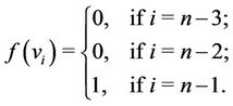
When the first and the last vertices of  are merged then
  becomes
 . In [2], Bertossi and Bonuccelli showed that
  is equal to 1 if n is multiple of 4 and 2 otherwise.
For complete graph , it is easy to check that
 .
.
The wheel , is obtained by joining
  and
and , i.e.,
 . It is also easy to check that
  .
.
Bertossi and Bonuccelli [2] investigated the  - labelling problem on complete binary trees, proving that 3 labels suffice. An optimum labelling as follows can be found. Assign first labels 0, 1 and 2, respectively, to the root, its left child and its right child. Then, consider the nodes by increasing levels: if a node has been assigned label
 , then assign the remaining labels to its grandchildren, but giving different to brother grandchildren. The above procedure can be generalized to find an optimum
  -labelling for complete (
 )-ary trees, requiring span
 . It is straight forward to see that when
  and
and  this result gives the
  - number for complete binary trees and paths respectively.
It is shown in [5] that for any tree ,
,  is equal to
 , implying that
 . An optimal
  -labelling can be also determined by exploiting the algorithm provided in [6] for optimally
  - labelling trees.
Bodlaender et al. [7] compute upper bounds for graphs of treewidth bounded by  proving that
 . They give also approximation algorithms for the
  - labelling running in
  time.
time.
In [2], the NP-completeness result for the decision version of the  -labelling problem is derived when the graph is planar by means of a reduction from 3-VERTEX COLORING of straight-line planar graph. An exhausted survey on
  -labelling is available in [8].
In [7], an approximation algorithm is designed for  -labelling a permutation graph in
  time; it guarantees the bound
 .
.
The n-dimensional hypercube  is an
is an  -regular graph with
  nodes. Then
  and there exists a labelling scheme using such a number of labels. This labelling is optimal when
  for some
  and it is a 2-approximation otherwise [9]. For a bipartite graph,
  [7]. Later this lower bound has been improved by a constant factor of
  [10]. A study on
  -labelling of cartesian product of a cycle and path is done by Chiang and Yan [11].
When  and
and  then we get
  -labelling problem. This problem was introduced by Grrigs and Yeh [12,13] in connection with the problem of assigning frequencies in a multihop radio network. Some results of
  -labelling problem are given below.
Kral and Skrekovski [14] improve the upper bound for any graph ,
, . The best known result till date is
  due to Goncalves [15].
Heuvel and Mc Guinness showed that  [16] for planar graphs. Molloy and Salavatipour [17] reduced this upper bound to
 . Wang and Lih [18] proved that if
  is a planar graph of girth (girth is defined to be the length of a shortest cycle in
 ) at least 5, then
In [19], we have showed that the upper and the lower bounds for  of a cactus graph
  is
is 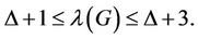
Adams et al. [20], give different bounds for certain generalized petersen graphs. A study on  -labelling of cartesian product of a cycle and a path is done by Chiang and Yan [11].
For further studies on the  -labelling, see [21- 30].
When  and
and  then we get another special case which is called
  -labelling problem. Some results of
  -labelling problem are given below.
For path, 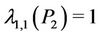 and
and 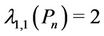 for each
 , and
, and  is 2 if
  is a multiple of 3 and it is 3 otherwise [31].
3. The L(0,1)-Labelling of Induce Sub-Graphs of Cactus Graphs
Let  be a given graph and subset
  of
of . The induced subgraph by
 , denoted by
  is the graph given by
 , where
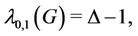
  . Some induced subgraphs of cactus graph are shown in Figure 1.
The cactus graphs have many interesting subgraphs, those are illustrated below. An edge is nothing but ,
,
 (a) (b) (c) (d)
Figure 1. Some induce subgraphs of cactus graph.
so . The star graph
  is a subgraph of cactus graph, therefore, one can conclude the following result.
Lemma 1. For any star graph 
 (1)
(1)
4. L(0,1)-Labelling of Cycles
In [2], Bertossi and Bonuccelli have labeled  by
by  -labelling and they have obtained the following result. Here we have given a constructive prove of this result.
4.1. L(0,1)-Labelling of One Cycle
Lemma 2. [2] For any cycle  of length
 ,
,
 (2)
(2)
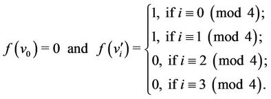
Proof. Let  be the vertices of the cycle
 . We classify
  into five groups, viz.,
  ,
,  ,
,  ,
,  and
and .Then the
  -labelling of the vertices of a cycle are as follows.
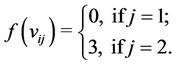
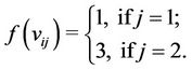
Case 1. Let .
.
Case 2. Let  (mod 4), i.e.,
 .
.
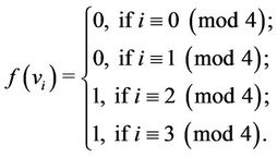
Case 3. Let  (mod 4), i.e.,
 .
.
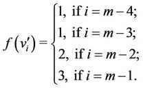
The label of first  vertices
  are same as in Case 2. For the last vertex
 ,
,  is define as
Case 4. Let  (mod 4), i.e.,
 .
.
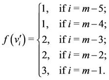
Here the label of first 4k + 1 vertices 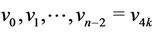 are same as in Case 3. For the last vertex
 ,
,  is define as

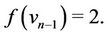
Case 5. Let  (mod 4), i.e.,
 .
.
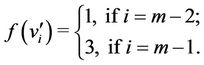
The label of first  vertices
 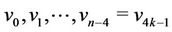 are same as in Case 2. For the last three vertices
 ,
,  ,
,  ,
,  is define as
Thus, from all above cases, we conclude that
4.2. L(0,1)-Labelling of Two Cycles
Lemma 3. Let G be a graph which contains two cycles and they have a common cutvertex. If  be the degree of G, then
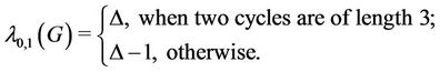 (3)
(3)
Proof. Let  contains two cycles
  and
and  of lengths
  and
and  respectively. Let
  be the cutverx and
  be the degree of
 . Let
. Let  and
and  be the vertices of
  and
and  respecvely. The labelling procedure of
 ’s of
’s of  of same as given in Lemma 2. Now we label the cycle
  as follows.
Case 1. Let  and
and .
.
The label of the cutvertex  is 0, i.e.,
 . The label of other vertices of
  are as follows:

Case 2. For  (mod 4) and
 .
.

Case 3. For  (mod 4) and
 .
.
Case 4. For  (mod 4) and
 .
.
The label of the vertices of  are same as given in Case 3 of that lemma.
Case 5. For  (mod 4) and
In this case, we label the of  as given in Case 3.
Case 6. For  (mod 4) and
 .
.
Here we label the adjacent vertices of  by
by  and
and . Now we label the other vertices
  of
of  as follows.

The above  is redefine for the vertex
  as
as
 .
.
In particular when , then we label the vertices of
  as follows.
The label of the cutvertex  and two adjacent vertices
  and
and  are same as above. And we label the remaining vertex
  by
by .
.
Case 7. For  (mod 4) and
  (mod 4).
Here the label of two vertices ,
,  of
of  are same as given in the above case. Now we label the vertices
  as
as

For the vertices  and
and ,
,  is defined as
  and
and 
In particular when , then we label the vertices of
  as follows.
The label of the cutvertex  and two adjacent vertices of
  of
of  are same as above. Now we label the remaining vertices of
  as
as

Case 8. For  (mod 4) and
 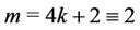 (mod 4).
The label of  of
of  are same as in above case. For the vertex
 , we label it as
 .
.
When , then the label of the vertices
 ,
,  ,
,  ,
,  and
and  are same as in the above case, and
 .
.
Case 9. For  (mod 4) and
  (mod 4).
We label the vertices of  and the vertices
 ,
,  ,
,  ,
,  and
and  of
of  according to the Case 8. For the vertex
 ,
,  is
is
In particular, when , the the label of the vertices of
  are same as the label of the vertices of
  as in the above case except the vertex
 . The label of the vertex
  is
is 
Case 10. For  (mod 4) and
  (mod 4).
We label first  vertices
 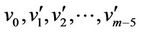 of
of  as
as

For the last four vertices ,
,  ,
,  and
and , the above
  is define as
In particular when , the label of the vertices
 ,
,  ,
,  and
and  are same as the label of the vertices
  shown above.
Case 11. For  (mod 4) and
  (mod 4).
We label first  vertices
  of
of  as per Case 10. And for the last five vertices,
  is define as
In particular when  then the label of the vertices
  are same as the label of the last five vertices of
  of the above case.
Case 12. For  (mod 4) and
  (mod 4).
Now we label first  vertices of
  as
as
For the last two vertices  and
and , the
, the  is
is
Case 13. For  (mod 4) and
  (mod 4).
Here we label the other vertices of  as in Case 11.
Case 14. For  (mod 4) and
  (mod 4).
In this case, the label of  are same as in Case 12.
Case 15. For  (mod 4) and
  (mod 4).
We label the vertices of  as per Case 12.
Thus from the above cases, it follow that

4.3. L(0,1)-Labelling of Three Cycles
Lemma 4. Let G be a graph, contains three cycles and they have a common cutvertex . If
. If  be the degree of
 , then,
 (4)
(4)
Proof. Let ,
,  and
and  be three cycles join by a common cutvertex
 , of lengths
 ,
,  and
and  respectively. Let
  be the degree of the cutvertex, i.e.,
 . Let
. Let ,
,  ,
,  ,
, ;
; ,
,  ,
,  ,
, ;
; ,
,  ,
,  ,
,  be the vertices of the cycles respectively.
Now we label the graph as follows.
Case 1. Let ,
,  and
and .
.
In Case 1 of Lemma 3, we label a graph which contains two cycles of length three and they have a common cutvertex . According to the previous lemma we label the vertices of the third cycle of length 3 as follows:
Case 2. For ,
,  ,
,  , where
  .
.
All the subcases of this case, the label of two vertices  and
and  of the cycle
  are
are
and the label of other two cycles are of different types, they are discussed below.
When  (mod 4) and
 .
.
Here the label of the vertices of the cycles  and
and , joined with a common cutvertex
  are same as in Case 2 of Lemma 3.
When  (mod 4) and
 .
.
The label of the vertices of  and
and  are same as in Case 3 of Lemma 3.
When  (mod 4) and
 .
.
The label of the vertices of  and
and  are same as in Case 4 of Lemma 3.
When  (mod 4) and
 .
.
We label the vertices of  and
and  as in Case 5 of Lemma 3.
Case 3. For ,
,  ,
,  , where
  .
.
In all subcases of this case, the label of three vertices of  are
are

And the label of the vertices of first two cycles  and
and  are same as in Case 6, Case 7, ..., Case 15, respectively of Lemma 3.
Case 4. For ,
,  ,
,  (mod 4), where
 .
.
For all subcases of this case, we label the vertices of the third cycle  as same as the labelling of the vertices of
  in Case 6 of Lemma 3 except two vertices
  and
and  (the adjacent vertices of
 ). Then we label these vertices as
  and
and .
.
And we label the first two cycles  and
and  (joined by a common cutvertex
 ), as same as in Case 6, Case 7, ..., Case 15 of Lemma 3.
Case 5. For ,
,  ,
,  (mod 4), where
 .
.
In all subcases of this case, we label the vertices of the third cycle  using the same process to labelling the vertices of
  in Case 7 of Lemma 3 except two vertices
  and
and  (the adjacent vertices of
 ). Now we label the adjacent vertices of
  of
of  as
as  and
and .
.
And we label the first two cycles  and
and  (joined by a common cutvertex
 ), as same as in Case 10, Case 11, ..., Case 15 of Lemma 3.
Case 6. For ,
,  ,
,  (mod 4), where
 .
.
In all subcases of this case, we label the vertices of the third cycle  using the same process of labelling of the vertices of
  in Case 7 of Lemma 3, except two vertices
  and
and . The label of
  and
and  are
are  and
and .
.
And the label of the vertices of the cycles  and
and  are same as in Case 13, Case 14 and Case 15 respectively of Lemma 3.
Case 7. For  (mod 4),
  (mod 4),
  (mod 4).
The label of the vertices of  and
and  are same as in Case 15 of Lemma 3. Here
 . Then we label the vertices of
  using the same process of
  in Case 9 of Lemma 3 except the vertices
  and
and . We label these vertices as
  and
and . Thus from all above cases, it follow that

4.4. L(0,1)-Labelling of Four Cycles
Using th results from Lemma 3 and Lemma 4 we can write the following statement.
Lemma 5. Let G be a graph which contains four cycles of any length and they have a common cutvertex. Then,
 (5)
(5)
where  be the degree of the cutvertex.
Corollary 1. Let G be a graph which contains finite number of cycles and they have a common cutvertex. If the vertices of the cycles (except the cutvertex) contain one or more edges then,
 (6)
(6)
4.5. L(0,1)-Labelling of Finite Number of Cycles
Let  be a graph which contains
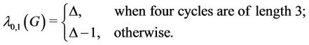
  number of cycles of length 3. Sometimes a cycle of length three is called triangle. A triangle is a subgraph of a cactus graph. Also, a triangle shaped star, (i.e., all the triangles that have a common cutvertex) is a subgraph of a cactus graph. Now, we consider a triangle shaped star for
  -labelling. Let
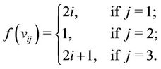
  be the
  triangles meet at a common cutvertex
  and we denote this graph by
 which is equivalent to
 . The number of vertices and edges of
  are
are  and
and  respectively. Again the graph
  may also contains
  number of cycles of finite length.
Then from Lemmas 3-5 we conclude the general form of these lemmas which is given below.
Lemma 6. Let the graph G contains n number of cycles of any length and they joined at a cutvertex, then
 (7)
(7)
where  be the degree of the cutvertex.
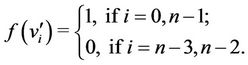
Proof. At first we prove that when  contains
  number of cycles of length 3 then the value of
  is
is , where
  be the degree of the graph. Let
  be the
  number of triangles joined with a common cutvertex
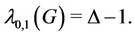
  (shown in Figure 2).
Let ,
,  and
and  be the vertices of
 , where
 . We label
  by 0.
by 0.
Then according to the previous lemmas the labels of

Figure 2. A graph contains n numbers of triangles.
 ’s are as follows.
For ,
,
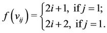
Now, the label of the vertex  of
of  is
is 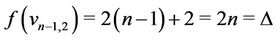 .
.
Therefore, 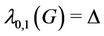 , when
  contains
  number of cycles of length 3.
Again, if we consider a graph  contains
  number of
  and
and  number of
 , then,
  , where
  be the degree of cutvertex, then the general form can be proved by mathematical induction, that is, when a graph
  contains finite number of cycles of any length then
 .
.
Let  contains
  number of
 ’s
’s  and
and  number of
 ’s
’s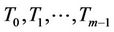 . Let
. Let  be the common vertex and degree of
  is
is . Again let
 ,
,  ,
,  ,
,  be the vertices of
  and
and ,
,  ,
,  be the vertices of
 . We label
  as 0. Then we label the other vertices of
 ’s as follows.
For 
and then the label of the vertices of ’s are given by.
For j = 0, 1, ···, n − 1,
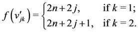
Now the label of third vertex of  is
is
Therefore, .
.
The general form can be proved by mathematical induction.
Hence the result.
Lemma 7. If a graph G contains finite number of cycles of any length and finite number of edges and they have a common cutvertex of degree , then
 (8)
(8)
Proof. Suppose that the lemma is true for  number of cycles of any length and
  number of edges. Now we have to prove that if we add a cycle of any length to the cutvertex then the value of
  for the new graph will be same, i.e., the value of
  will preserve for
  number of cycles of any length.
Now the graph  contains
  number of cycles of any length and
  number of edges joined with a common cutvertex
 . Then the degree of
  is
is . In the previous lemma we proved that when a graph contains finite number of cycles of any length then,
At first we prove that if  contains
  number of cycles of length 3 and
  number of edges then the value of
  for that graph remains same. When all cycles are of length 3 then according to the Lemma 5 the label of two vertices of
  th cycle of length 3 are as
where ,
,  and
and  are three vertices of
  th cycle. Let
 ,
, ;
; ,
, ;
; ;
; ,
,  are the vertices of
  edges. Here the label of the cutvertex
  is 0. Then we label the other vertices of the edges as follows

Now we add another cycle of length 3 to the cutvertex . Then the degree of
  is
is . Let
. Let ,
,  and
and  be the vertices of
  th cycle. We label the two vertices
  and
and  as
as

Here we see that the label of third vertex of  th cycle is
  as
as . That is, the value of
  of the graph which contains
  number of cycles of length 3 and
  number of edges is same.
Similarly, we can prove that the value of  will preserve for the graph which contains
  number of cycles and
  number of edges.
Hence the result.
5. L(0,1)-Labelling of Sun
Let us consider the sun  of
of  vertices. This graph is obtained by adding an edge to each vertex of a cycle
 . So
. So  is a subgraph of
 . But, what is the value of
Lemma 8. For any sun ,
,
 (9)
(9)
Proof. Let  be constructed from
  by adding an edge to each vertex. To label this graph we consider five cases.
Let  be the vertices of
  and
and  is adjacent to
  and
and . To complete
 , we add an edge (
 ,
, ) to the vertex
 , i.e.,
 ’s are the pendent vertices. The labelling procedure of
  is same as given in Lemma 2. Now we label the pendent vertices as follows.
Case 1. Let .
.
The label of  's are as
Case 2. Let  (mod 4).
The label of  are assigned as
  for
for .
.
Case 3. Let  (mod 4).
The label of the vertices ’s are given by
 ;
;  for
for  and
and  and
and .
.
Case 4. Let  (mod 4).
The label of the vertices  's are given by
 , for
, for ;
;
 for
for ;
;
 , for
, for .
.
Case 5. Let  (mod 4).
In this case the label of the pendent vertices  's are as follows:
 , for
, for ;
;
 ;
; , for
, for .
.
Hence .
.
Lemma 9. Let  be a graph obtained from
  by adding an edge to each of the pendent vertex of
 , then
 (10)
(10)
Proof. Let the graph is obtained by adding an edge  to each of the pendent vertices
  s. So in the new graph
  are the pendent vertices.
Case 1. Let .
.
 ,
,  , for
, for .
.
Case 2. Let  (mod 4).
 , for
, for .
.
Case 3. Let  (mod 4).
 ,
,  and
and , for
, for 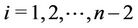 .
.
Case 4. Let  (mod 4).
and , for
, for .
.
Case 5. Let  (mod 4).
 , for
, for , and
, and , for
, for .
.
Thus, from all above cases we have
 .
.
Lemma 10. If the graph  contains a cycle of any length and each vertex of the cycle has another cycle of any length, then
 (11)
(11)
where  is the degree of
 .
.
Proof. At first we prove that if the graph  contains a cycle
  of length
  and each vertex of
  contains another cycle of length 3, or length 3 and length 4, or length 4, then
  or
or . Let
. Let  be the vertices of
  and
and ;
; ;
; ;
;  are the vertices of all
 ’s which are joined with each vertex of
 . If the vertex
  of
of  contains a cycle of length 4 then let the vertices of
  be
be ,
,  and
and . Again if the vertex
  contains a cycle of length 4 then let the vertices of
  be
be ,
,  and
and . Therefore, all the vertices of
  are cutvertices.
Now we label the graph as follows.
Case 1. For .
.
Now, we label the vertices of other cycles joined with the vertices of  according to the following rule
If there are three cycles of length 4 then we label the vertices as follows:

and 
Case 2. Let  (mod 4).
For ,
,

If all other cycles are of length 4 then the label of the last vertex of the last cycle is 3.
Case 3. Let  (mod 4).


and 
If the ( )th vertex
  of
of  contains a cycle of length 4 then we label the vertices of
  as
as

Case 4. Let  (mod 4).
Now the label of all  's are as follows:
for ,
, 
for ,
, 
and for ,
, 
If  contain combined
  's and
  's then the minimum span is 3.
Case 5. Let  (mod 4).
For ,
, 

and for ,
, 
If the vertex  contains a cycle of length 4 then the label of the vertices adjacent to
  are
are

From all the above cases, we see that 3 or 4 are used to label , which is equal to
  or
or .
.
Therefore, .
.
The proves of the other cases are similar.
Corollary 2. Let G be a graph which contains a cycle of length . If each vertex of the cycle contains two or more cycles of length more than 2, then
 (12)
(12)
where  be the degree of G.
6. L(0,1)-Labelling of Caterpillar Graph
Now, we label another important subclass of cactus graphs called caterpillar graph.
Definition 1. A caterpillar  is a tree where all vertices of degree
  lie on a path, called the backbone of
 . The hairlength of a caterpillar graph
  is the maximum distance of a non-backbone vertex to the backbone.
Lemma 11. If G be a caterpillar graph and  be its degree, then
 (13)
(13)
Proof. Let  be a path of length
  of the caterpillar graph and
  be the vertices of
 . We label the vertices of
  according to the following rule.

Let us assume that  be any vertex of
  and
and ,
,  are the adjacent vertices of
 . As we label of the vertices of
  by 0 or 1 so without loss of generality let us consider that the label of
 ,
,  and
and  are 0, 0 and 1 respectively. Again let us consider that
  number of paths
 ;
; , of same lengths are joined to the vertex
 . Let
. Let ;
; 
 are the vertices of
  paths other than
 . Now we label the vertices of these paths as in the following method:
 for
for  and
and .
.
And we label other vertices of  's as per the rule to label the vertices of
 .
.
Now, .
.
The result will be same when finite number of paths of different lengths are joined to one or more vertices of the path of the caterpillar graph.
So, .
.
7. L(0,1)-Labelling of Lobster
Another subclass of cactus graphs is the lobster graph. The definition of lobster graph is given below.
Definition 2. A lobster is a tree having a path (of maximum length) from which every vertex has distance at most , where
  is an integer.
The maximum distance of the vertex from the path is called the diameter of the lobster graph. There are many types of lobsters given in literature like diameter 2, diameter 4, diameter 5, etc.
Lemma 12. Let G be a lobster graph. If  be the degree of the lobster graph, then
 (14)
(14)
Proof. Let  be a path of length
  of the lobster graph and
  be the vertices of
 . First we label the vertices of
  according to Lemma 11.
Then we label the other vertices of that graph. Let us denote the other vertices of the graph by . Here
  are adjacent to
  and
and ,
, . The label of the vertices of
  are either 0 or 1. Then we label the vertices
  by 2, 3 and so on [it depends upon (
 )].
)].
Thus the  -value of a lobster is
 .
.
We know from [2] that 3 labels are sufficent to label a complete binary tree by  -labelling. Now we have to prove that for any tree the value of
  is
is , where
  is the degree of the tree.
Lemma 13. For any tree  of degree
 ,
,
 (15)
(15)
Proof. Let  be a tree with degree
 . We first label the root of the tree by 0. Now we know from the definition of
  -labelling that the label difference between any two adjacent vertices is at least 0 and the label difference between any two vertices which are at distance two is at least 1. Now we label the children of the root from left to right by 0, 1, 2,
  ,
, .
.
Let us consider the  th vertex of the tree. Assume that the label of the parent of
  is known. Then the allowable label for the children of
  are 0, 1, 2,
  except the label of the parent of
 . Now, we label the children of
  by 0, 1, 2,
  ,
,  ,
,  , where
  is the degree of the vertex
 , except the label of the parent of
 . This process is valid for any vertex
  of the tree. Thus the maximum label used to label the entire tree by
  -labelling is max{
 :
:  }, which is exactly equal to
 .
.
Hence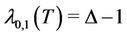 .
.
The  -labelling of all subgraphs of cactus graphs and their combinations are discussed in the previous lemmas. From these results we conclude that the
  -value of any cactus graph can not be more than
 . Hence we have the following theorem.
Theorem 1. If  is the degree of a cactus graph
 , then
 (16)
(16)
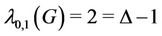
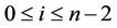
The graph of Figure 3 is an example of a cactus graph, contains all possible subgraphs and its  -labelling.
8. Conclusion
The bounds of  -labelling of a cactus graph and various subclass viz., cycle, sun, star, caterpillar, lobster and tree are investigated. The bounds of
  for these graphs are
  or 2, for sun, star, caterpillar, lobster and tree it is
 . For the cactus graph the bound is
 , where
  is the
Figure 3. L(0,1)-labelling of a cactus graph.
maximum degree of the cactus graph . Currently we are engaged to find the bounds for
  -labelling for different values of
 ,
,  on cactus graphs.
REFERENCES
- W. K. Hale, “Frequency Assignment: Theory and Applications,” Proceedings of IEEE, Vol. 68, No. 12, 1980, pp. 1497-1514. doi:10.1109/PROC.1980.11899
- A. A. Bertossi and M. A. Bonuccelli, “Code Assignment for Hidden Terminal Interference Avoidance in Multihope Packet Radio Networks,” IEEE/ACM Transactions on Networking, Vol. 3, No. 4, 1995, pp. 441-449. doi:10.1109/90.413218
- X. T. Jin and R. K. Yeh, “Graph Distance-Dependent Labelling Related to Code Assignment in Compute Networks,” Naval Research Logistics, Vol. 51, 2004, pp. 159-164.
- T. Makansi, “Transmitter-Oriented Code Assignment for Multihop Packet Radio,” IEEE Transactions on Communications, Vol. 35, No. 12, 1987, pp. 1379-1382. doi:10.1109/TCOM.1987.1096728
- J. P. Georges and D. W. Mauro, “Generalized Vertex Labeling with a Condition at Distance Two,” Congressus Numerantium, Vol. 140, 1995, pp. 141-159.
- A. A. Bertossi, M. C. Pinotti and R. Rizzi, “Channel Assignment on Strongly-Simplicial Graphs,” IEEE Proceedings of International Parallel and Distributed Processing Symposium (IPDPS’03), Nice, 22-26 April 2003, pp. 22-26.
- H. L. Bodlaender, T. Kloks, R. B. Tan and J. Van Leeuwen, “Approximations for λ-Colorings of Graphs,” The Computer Journal, Vol. 47, No. 2, 2004, pp. 193-204. doi:10.1093/comjnl/47.2.193
- T. Calamoneri, “The L(h, k)-Labelling Problem: A Survey and Annotated Bibliography,” The Computer Journal, Vol. 49, No. 5, 2009, pp. 585-630. doi:10.1093/comjnl/bxl018
- P. J. Wan, “Wear-Optimal Conflict-Free Channel Set Assignments for an Optical Cluster-Based Hypercube Network,” Journal of Combinatorial Optimization, Vol. 1, 1997, pp. 179-186. doi:10.1023/A:1009759916586
- N. Alon and B. Mohar, “The Chromatic Number of Graph Powers,” Combinatorics, Probability and Computing, Vol. 11, No. 1, 2002, pp. 1-10. doi:10.1017/S0963548301004965
- S. H. Chiang and J. H. Yan, “On L(d, 1)-Labeling of Cartesian Product of a Path,” Discrete Applied Mathematics, Vol. 156, No. 15, 2008, pp. 2867-2881. doi:10.1016/j.dam.2007.11.019
- J. R. Griggs and R. K. Yeh, “Labeling Graphs with a Condition at Distance 2,” SIAM Journal on Discrete Mathematics, Vol. 5, No. 4, 1992, pp. 586-595. doi:10.1137/0405048
- R. K. Yeh, “Labeling Graphs with a Condition at Distance Two,” Ph.D Thesis, University of South Carolina, Columbia, 1990.
- D. Kral and R. Skrekovski, “A Theorem on Channel Assignment Problem,” SIAM Journal on Discrete Mathematics, Vol. 16, No. 3, 2003, pp. 426-437. doi:10.1137/S0895480101399449
- D. Goncalves, “On the L(p,1)-Labelling of Graphs, in: EuroCom 2005,” Discrete Mathematics and Theoretical Computer Science Proceedings, Vol. AE, 2005, pp. 81-86.
- J. Van den Heuvel and S. McGuinnes, “Coloring the Square of a Plannar Graph,” Journal of Graph Theory, Vol. 42, No. 2, 2003, pp. 110-124. doi:10.1002/jgt.10077
- M. Molloy and M. R. Salavatipour, “A Bound on the Chromatic Number of the Square of a Planar Graph,” Journal of Combinatorial Theory, Series B, Vol. 94, No. 2, 2005, pp. 189-213. doi:10.1016/j.jctb.2004.12.005
- W. F. Wang and K. W. Lih, “Labelling Planar Graphs with Conditions on Girth and Distance Two,” SIAM Journal on Discrete Mathematics, Vol. 17, 2004, pp. 499-509.
- N. Khan, A. Pal and M. Pal, “L(2,1)-Labelling of Cactus Graphs,” Communicated.
- S. S. Adams, J. Cass, M. Tesch, D. S. Troxell and C. Wheeland, “The Minimum Span of L(2,1)-Labeling of Certain Generalized Petersen Graphs,” Discrete Applied Mathematics, Vol. 155, No. 1, 2007, pp. 1314-1325. doi:10.1016/j.dam.2006.12.001
- G. J. Chang, W. T. Ke, D. Kuo, D. D. F. Lin and R. K. Yeh, “On L(d,1)-Labellings of Graphs,” Discrete Mathematics, Vol. 220, 2000, pp. 57-66. doi:10.1016/S0012-365X(99)00400-8
- G. J. Chang and C. Lu, “Distance Two Labelling of Graphs,” European Journal of Combinatorics, Vol. 24, 2003, pp. 53-58. doi:10.1016/S0195-6698(02)00134-8
- J. Fiala, T. Kloks and J. Kratochvil, “Fixed-Parameter Complexity of λ-Labelling,” Discrete Applied Mathematics, Vol. 133, No. 1, 2001, pp. 59-72. doi:10.1016/S0166-218X(00)00387-5
- J. Georges and D. W. Mauro, “On Generalized Petersen Graphs Labelled with a Condition at Distance Two,” Discrete Mathematics, Vol. 259, No. 1-3, 2002, pp. 311- 318. doi:10.1016/S0012-365X(02)00302-3
- J. Georges, D. W. Mauro and M. I. Stein, “Labelling Products of Complete Graphs with a Condition at Distance Two,” SIAM Journal on Discrete Mathematics, Vol. 14, 2000, pp. 28-35. doi:10.1137/S0895480199351859
- P. K. Jha, “Optimal L(2,1)-Labelling of Cartesian Products of Cycles with an Application to Independent Domination,” IEEE Transactions on Circuits and Systems I: Fundamental Theory and Applications, Vol. 47, No. 10, 2000, pp. 1531-1534. doi:10.1109/81.886984
- S. Klavzar and A. Vesel, “Computing Graph Invariants on Rotagraphs Using Dynamic Algorithm Approach: The Case of L(2,1)-Colorings and Independence Numbers,” Discrete Applied Mathematics, Vol. 129, 2003, pp. 449- 460. doi:10.1016/S0166-218X(02)00597-8
- D. Kuo and J. H. Yan, “On L(2,1)-Labelling of Cartesian Products of Paths and Cycles,” Discrete Mathematics, Vol. 283, No. 1-3, 2004, pp. 137-144. doi:10.1016/j.disc.2003.11.009
- C. Schwarz and D. S. Troxell, “L(2,1)-Labelling of Products of Two Cycles,” Discrete Applied Mathematics, Vol. 154, No. 1-3, 2006, pp. 1522-1540. doi:10.1016/j.dam.2005.12.006
- R. K. Yeh, “The Edge Span of Distance Two Labelling of Graphs,” Taiwanese Journal of Mathematics, Vol. 4, No. 4, 2000, pp. 675-683.
- R. Battiti, A. A. Bertossi and M. A. Bonuccelli, “Assigning Code in Wireless Networks: Bounds and Scaling Properties,” Wireless Networks, Vol. 5, No. 3, 1999, pp. 195-209. doi:10.1023/A:1019146910724