Communications and Network
Vol.3 No.2(2011), Article ID:4968,7 pages DOI:10.4236/cn.2011.32009
The Symbolic OBDD Algorithm for Finding Optimal Semi-Matching in Bipartite Graphs
School of Computer Science, Guilin University of Electronic Technology, Guilin, China
E-mail: gu@guet.edu.cn
Received December 2, 2010; revised January 19, 2011; accepted February 28, 2011
Keywords: Bipartite Graphs, Semi-Matching, Load Balancing, Ordered Binary Decision Diagram
Abstract
The optimal semi-matching problem is one relaxing form of the maximum cardinality matching problems in bipartite graphs, and finds its applications in load balancing. Ordered binary decision diagram (OBDD) is a canonical form to represent and manipulate Boolean functions efficiently. OBDD-based symbolic algorithms appear to give improved results for large-scale combinatorial optimization problems by searching nodes and edges implicitly. We present novel symbolic OBDD formulation and algorithm for the optimal semimatching problem in bipartite graphs. The symbolic algorithm is initialized by heuristic searching initial matching and then iterates through generating residual network, building layered network, backward traversing node-disjoint augmenting paths, and updating semi-matching. It does not require explicit enumeration of the nodes and edges, and therefore can handle many complex executions in each step. Our simulations show that symbolic algorithm has better performance, especially on dense and large graphs.
1. Introduction
The matching problems arise in many practical application settings where we often wish to find the proper way to pair objects or people together to achieve some desired goal. Also the search for certain matching can be an important subtask for some complex problems such as the maximum network flow and traveling salesman problem [1]. The matching problems were classified into the followings [2]. Problem 1 (Maximum Cardinality Matching in Bipartite Graphs): The nodes are partitioned into boys and girls, and an edge can only join a boy and a girl. We look for a matching with the maximum cardinality. Problem 2 (Maximum Cardinality Matching in General Graphs): This is the asexual case, where an edge joins two persons. Problem 3 (Maximum Weighted Matching in Bipartite Graphs): Here we still have nodes representing boys and girls, but each edge has a weight associated with it. Our goal is to find a matching with the maximum total weight. This is the well-known assignment problem of assigning people to jobs and maximizing the profit. Problem 4 (Maximum Weighted Matching in General Graphs): This problem is obtained from Problem 1 by making it harder in both ways. Formally, a bipartite graph is a graph G = (U ÈV, E) in which U ÇV = Æ and E Í U ´ V. A matching in G is a set of edges, M Í E, such that each node in U È V is an endpoint of at most one edge in M. In other words, each node in U is matched with at most one node in V and vice-versa. Maximum cardinality matching problem in bipartite graph is finding a matching that contains a maximum number of edges, and many efficient polynomial algorithms for computing the solutions have been developed [1,2].
The load balancing problems have received intense study in operations research and industrial engineering, in which we are given a set of tasks and a set of machines, each machine can process a subset of the tasks, and each task requires one unit of processing time. We need assign each task to some machines that can process it in a manner that minimizes some optimization objective. One possible objective is to minimize the makespan of the schedule, which is the maximal number of tasks assigned to any given machine. Another possible goal is to minimize the average completion time, or flow time, of the tasks. A third possible goal is to maximize the fairness of the assignment from the machines’ point of view, i.e., to minimize the variance of the loads on the machines. Motivated by load balancing problem, Harvey et al. defined the optimal semi-matching problem through relaxing maximum cardinality matching in bipartite graphs [3]. Formally, a semi-matching in a bipartite graph G = (U ÈV, E) is a set of edges, M Í E, such that each node in U is an endpoint of exactly one edge in M. Clearly a semi-matching does not exist if there are isolated nodes in U, so we require that each node in U have degree at least 1. Note that it is trivial to find a semi-matching, i.e., simply match each node in U with an arbitrary neighboring node in V. Harvey et al.’s optimal semi-matching problem is finding a semi-matching that match U with V as fairly as possible, that is, minimizing the variance of the matching edges at each V-node. To compute optimal semi-matching efficiently, they presented two algorithms. The first algorithm generalizes the Hungarian method for computing maximum bipartite matching, and the second one is based on the notion of cost-reducing paths. Experimental results demonstrated that the second algorithm is vastly superior to using known network optimization algorithms to solve the optimal semi-matching problem [3]. The concept of semi-matching appeared firstly in Lawler’s book [4], with the objective of finding maximum weight subset of elements in a matrix.
Finding optimal semi-matching in bipartite graphs is one of typical combinatorial optimization problems, where the size of graphs is a significant and often prohibitive difficulty. This phenomenon is known as combinatorial state explosion, resulting in that large graphs cannot be stored and operated on even the largest contemporary computers. In recent years, implicitly symbolic representation and manipulation technique, called as symbolic graph algorithm or symbolic algorithm [5,6], has emerged in order to combat or ease combinatorial state explosion. Typically, ordered binary decision diagram (OBDD) or variants thereof are used to represent the discrete objects [6-9]. Efficient symbolic algorithms have been devised for hardware verification, model checking, testing and optimization of circuits [7,8]. Hachtel and Somenzi developed OBDD-based symbolic algorithm for maximum flow in 0-1 networks that can be applied to very large graphs (more than 1036 edges) [10]. Gu and Xu presented the symbolic ADD (Algebraic Decision Diagram) formulation and algorithms for maximum flow problems in general networks [11]. Symbolic algorithms appear to be a promising way to improve the computation of large-scale combinatorial optimization problems through encoding and searching nodes and edges implicitly. Our contribution is to present the symbolic algorithm for optimal semi-matching in bipartite graphs.
The rest of this paper is organized as follows. In Section 2, we introduce some concepts and properties regarding bipartite graphs and maximum cardinality matching. The symbolic formulations for bipartite graphs and optimal semi-matching are described in Section 3; Section 4 presents the symbolic OBDD algorithm; The last Section gives experimental results and analysis.
2. Preliminaries
Given a graph G = (V, E) where V is a set of nodes with  and E a set of edges with
 , a matching M of G is a subset of edges set E such that no two elements of M are incident to the same node. We refer to the edges in M as matched edge, and edges not in M as unmatched or free edges. We also refer to a node v Î V as matched node with respect to a matching M if there is an edge in M incident to v, and it is called free or unmatched otherwise. For a matched node v the unique node w connected to v by a matching edge is called the mate of v. The cardinality
  of a matching M is the number of edges in M. A matching which contains a maximum number of edges is called the maximum-cardinality matching of the graph.
A simple path p in G is called an alternating path with respect to the matching M if the edges in p are alternately in M and not in M. If an alternating path starts and ends at the same node, it is called as an alternating cycle. We refer to an alternating path as an even alternating path if it contains an even number of edges and an odd alternating path if it contains an odd number of edges. An odd alternating path with respect to a matching M is called as an augmenting path if the first node and last node in the path p are unmatched or free.
Property 1 If p is an augmenting path with respect to a matching M, then  = (M − p)È(p − M) is also a matching of cardinality |M| + 1. Moreover, in the matching
 , all the matched nodes in M remain matched, and two additional nodes, namely the first and last nodes of p, are matched.
Property 2 If  holds for two matching M1 and M2 of G, then there are d (=
 ) augmenting paths with respect to M1 in G, and the paths are node-disjoint.
A bipartite graph G = (U ÈV, E) is a graph whose node set is partitioned into two non-empty disjoint groups U and V (U ∩ V= Æ) such that every edge of the graph is incident on at most one node from each group. This particular structure of bipartite graphs can be used in developing the algorithms for maximum cardinality matching. We can direct all unmatched edges from U to V and all matched edges from V to U, and refer to the directed bipartite graph (U È V, E¢) as a residual network with respect to bipartite graph G and matching M. On the directed view, the existence of an augmenting path is then tantamount to the existence of a path from a free node in U to a free node in V. Also, augmenting by a path p is trivial. One simply reverses the direction of all edges on the path. Observe that this correctly records that the endpoints of p are now matched and that M is replaced by . We will use this directed view in all our implementations of bipartite matching algorithms.
Property 2 guarantees the existence of many augmenting paths when current matching is still far from optimality, and suggests organizing many node-disjoint augmenting paths in each execution. In this regard, layered networks are usually constructed. In a layered network the nodes of a graph are partitioned into layers according to their distance with respect to the starting layer, i.e., a node v belongs to layer k if there is a path from the starting layer to v consisting of k edges and there is no path with fewer edges. For any edge in a layered network the distance of the target node is at most one more than the distance of the source node. The construction of the layered network begins by putting all free nodes in U into the zeroth layer, and proceeds by breadth-first search. The first layer is completed that contains free nodes in V, and the second layer contains free nodes in U and so on. Only edges that connect different layers can be contained in shortest augmenting paths, and the layered network contains all augmenting paths of shortest length.
3. Symbolic Formulation
An ordered binary decision diagram (OBDD) [5,6] provides compact, canonical and efficiently manipulative representation for Boolean functions. The OBDD for a non-constant Boolean function f is a directed acyclic graph G = (V, E). It includes sink or terminal nodes ‘0’ and ‘1’, which represent constant Boolean functions 0 and 1. These nodes have no descendants. All other nodes vÎV include a labeled variable l(v), and have two out-going edges of then and else cofactors drawn as solid and dash lines. The nodes are in one-to-one correspondence with Boolean functions. The function f(v) of a node vÎV is specified as l(v)×f(v)then+ l(v)¢×f(v)else, where “×” and “+” denote Boolean conjunction and disjunction respectively, and f(v)then and f(v)else are the functions of the then and else children. The root node of an OBDD represents the function f. The variables in an OBDD are ordered, i.e., if v is a descendant of u , which means (u, v) Î E, then l(u) < l(v), and all the paths in the OBDD keep the same variable ordering.
Given a Boolean function and any assignments to its variables, the function value is determined by tracing a path from the function node to a terminal node following the appropriate branch from each node. The branch depends on the variable value of the assignments, and the function value under the assignments is determined by its path’s terminal or sink node.
For example, Figure 1 shows the binary tree and the OBDD for Boolean function f = x1 × x3 + x2 × x3, where x1 < x2 < x3. It is obvious that the OBDD is a directed acyclic graph, and stores the same information in a more compact way. We trace the path ①®②®③®④, and reach the sink node 0. Thus, the value of Boolean function f = x1 × x3+x2 × x3 of variable assignment (0,1,0) is 0.
An important property of OBDDs is that they are a canonical representation of Boolean functions. Canonicity means that for a Boolean function f and each variable ordering p there is a unique OBDD, and vice versa. Moreover, many operations of Boolean functions can be implemented efficiently through graphical manipulations of OBDDs.
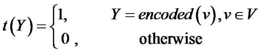
We convert a bipartite graph G = (U ÈV, E) to an OBDD by encoding the nodes of G with a length-n binary number, where n = . The ennode in U corresponds to a vector of binary variables X = (x0, ···, xn-1), and encoded node in V corresponds to a vector of binary variables Y = (y0, ···, yn-1). The edge (u, v)ÎE of G can be represented by binary vector (X, Y) = (x0, ···, xn-1, y0, ···, yn-1 ), where X = encoded (u) = (x0, ···, xn-1) and Y = encoded(v) = (y0, ···, yn-1) are the binary encoding of node u and v respectively. Thus, a bipartite graph is formulated by a triple (s(X), t(Y), E(X, Y)), where s(X), t(Y) and E(X, Y) are the characteristic functions as following:
 (3.1)
(3.1)
 (3.2)
(3.2)
(3.3)
These characteristic functions are of Boolean functions, and can be compactly represented by OBDDs. For example, an OBDD for the bipartite graph in Figure 2(a) is shown in Figure 2(b).
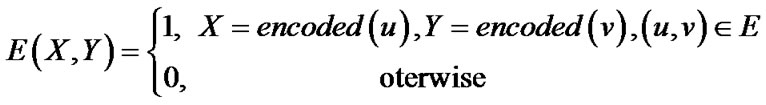
Given a bipartite graph (s(X), t(Y), E(X, Y)), the optimal semi-matching problem is formulated as follows:
max: (3.4)
(3.4)
subject to: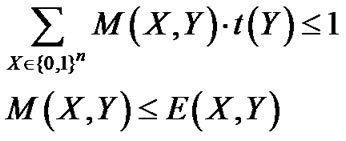 (3.5)
(3.5)
4. Symbolic OBDD Algorithm
Given the symbolic representation (s(X), t(Y), E(X, Y))for a bipartite graph G = (U ÈV, E), the pseudo-code of the symbolic OBDD algorithm for optimal semimatching is presented in Figure 3.
It begins by greedily searching initial matching and then iterates through a sequence of phases. Each phase consists of the following main steps: generating residual network; building layered network; traversing nodedisjoint augmenting paths; and updating semi-matching. The algorithm terminates and returns the maximum semi-matching when the cardinality  of semimatching M equals the cardinality
 . In the algorithm, variables and data are stored in OBDD forms, and computations are implemented by symbolic OBDD operations.
1) Searching initial matching through heuristic functions In order to obtain matching directly, we adopt a heuristic function P(X,Y,Z):{0,1}n×{0,1}n×{0,1}n ®{0,1}. The first argument is the base, and two other arguments are the nodes to be compared. For every choice of base X, P returns 1 if the second argument precedes the third one, else return 0.
Two different heuristic functions are used in the symbolic algorithm. The first one, relative proximity heuristic function, is PR(X,Y,Z) = ||Y-X||<||Z-X||, where ||X-Y|| = . The second is PD(X,Y,Z) = (||Y|| < ||Z||)called as datum proximity heuristic function that is a special case of relative proximity heuristic function independent of the base and simply returns the result of testing ||Y||<||Z||. Both heuristic functions can be represented by BDDs of size linear in n[10].
We obtain an initial matching of bipartite graph (s(X), t(Y), E(X, Y) by the following computation:
 (4.1)
(4.1)
The edges in Q(X,Y) form a right-unique relation, i.e., there is at most one edge out of each node X. MP(X,Y) is a left-unique subset of Q(X,Y), and consists of edges that share no end nodes.
For example, Figure 4(a) and 4(b) show the initial matching (darkened lines) of the bipartite graph in Figure 2(a) using relative proximity heuristic function and datum proximity heuristic function respectively. The heuristic functions are also applied in finding nodedisjoint augmenting paths.
2) Generating residual network In order to find a semi-matching that match U with V as fairly as possible, we rank the nodes in V by incident degrees in a semi-matching M, which is defined as following:
 (4.2)
(4.2)
The residual network under semi-matching M consists of unmatched nodes in U and nodes with the smallest degree in V. It is implemented by the following computations:

(4.3)
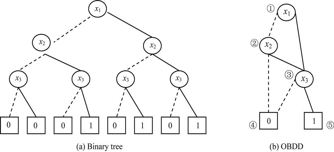
Figure 1. OBDD for boolean function f = x1 × x3 + x2 × x3.
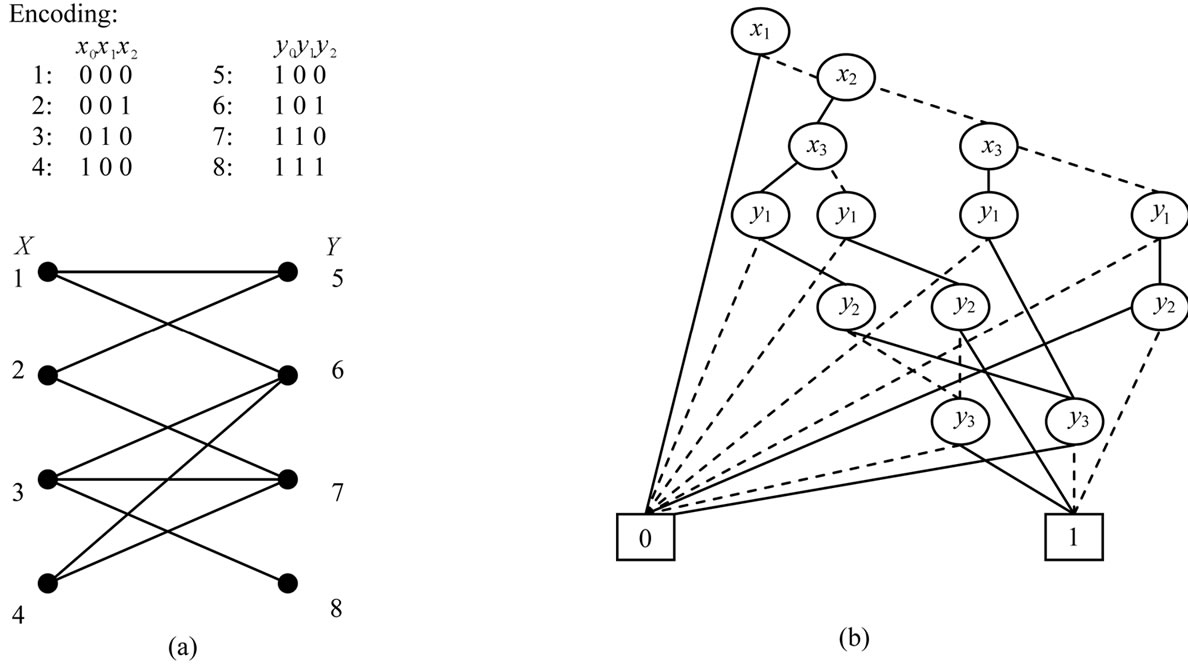
Figure 2. OBDD for a bipartite graph.
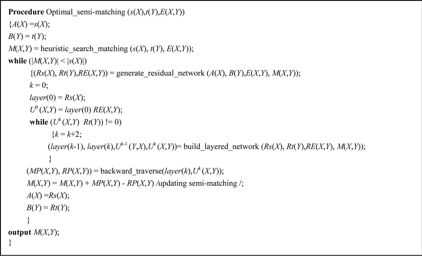
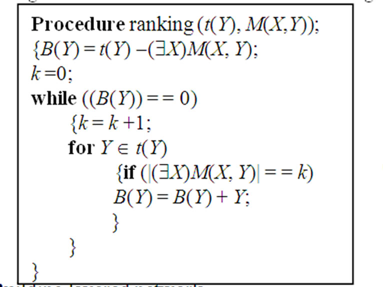
Figure 3. Pseudo-code for symbolic OBDD algorithm.
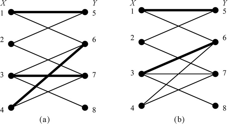
Figure 4. Heuristic search for initial matching.
 (4.4)
(4.4)
3) Building layered network We need to build the layered network from a residual network so as to obtain node-disjoint augmenting paths. We initialize layer zero by setting nodes layer(0) with Rs(X) and outgoing edges U(0)(X,Y) with layer(0)×RE(X,Y). On odd layer (2i+1), nodes layer (2i+1) are target-nodes from edges U(2i) (X,Y), and outgoing edges U(2i+1)(Y,X) include matched edges layer (2i+1)×RE(X,Y). Even layer 2i consists of nodes layer (2i) of target-nodes from edges U(2i-1) (Y,X) and outgoing edges U(2i)(Y,X) of unmatched edges layer(2i)×RE(X,Y). A layered network is built by forward-breadth-first traversing residual network. It is implemented by the following computations (Equation (4.5)).
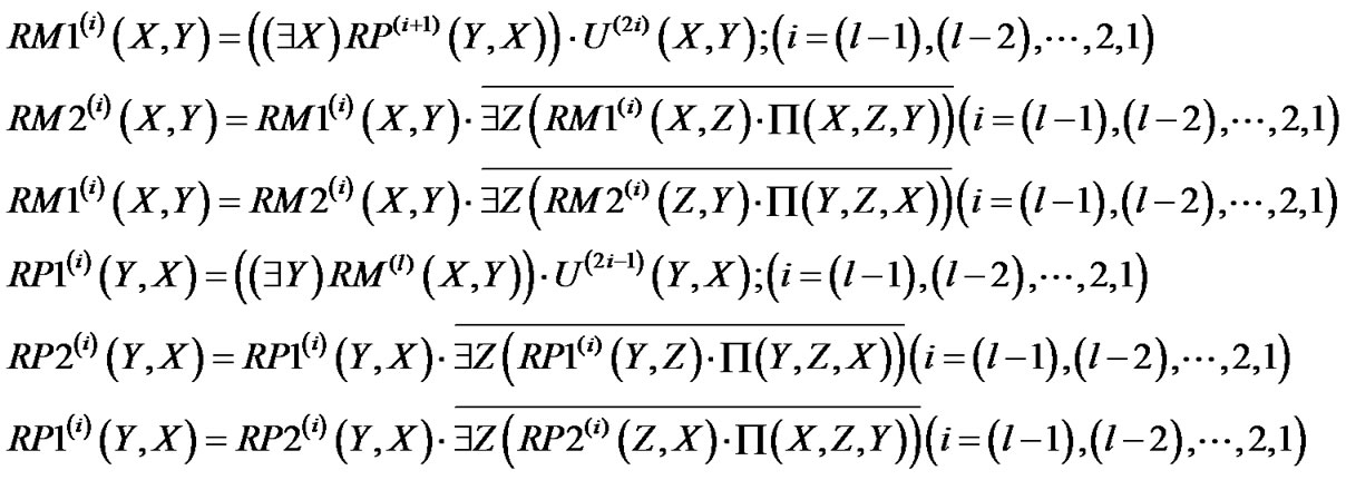
4) Backward traversing node-disjoint augmenting paths Once a layered network is constructed, we go through a series of steps to find node-disjoint augmenting paths. Supposed that the top layer of layered network with k = 2l layers satisfies  ¹ 0, i.e., layer(2l + 1) will have unmatched nodes, we proceed to build node-disjoint augmenting paths backward from unmatched edges RM(l) (Y,X) and matched edges RP(l)(X,Y) (Equation (4.6)).
Backward breadth-first traversing is implemented by the following computations (Equation (4.7)):
This process terminates by computing RM(0) (X,Y), resulting in node-disjoint MP(X,Y) and RP(X,Y). Heuristic functions guarantee that the augmenting paths are node (4.5)
(4.5)
 (4.6)
(4.6)
 (4.7)
(4.7)
 (4.8)
(4.8)
 (4.9)
(4.9)
disjoint and have the shortest length (Equation (4.8) and (4.9)).
5. Experimental Results
The symbolic OBDD algorithm proposed in this paper has been implemented in windows 2000 and software package CUDD [12]. Two groups of experiments are conducted. In both cases, CPU time is in seconds on a P4 1500MHz with 128MB of memory.
In the first group of experiments, the symbolic OBDD algorithm is compared with Asm1 and Asm2 algorithms [3]. We choose randomly generated graphs with different numbers of nodes and edges. Random graphs are very close to worst cases for symbolic algorithms. The results are shown in Table 1.
In the second group of experiments, we choose randomly generated graphs with 4000 nodes and different
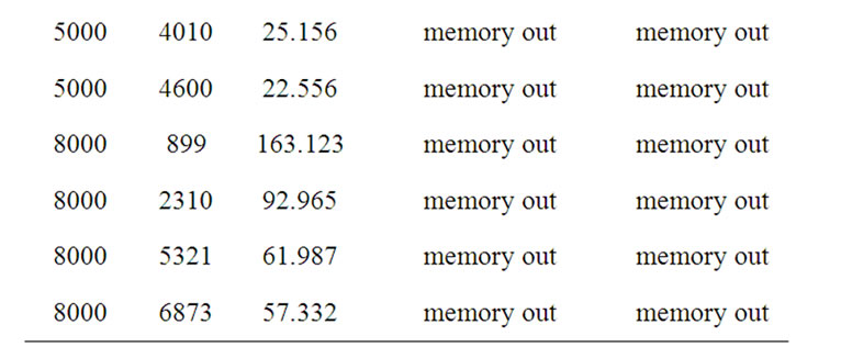

Table 1. Comparison of symbolic OBDD algorithm with Asm1and Asm2 algorithms.

Figure 5. Comparison of symbolic OBDD algorithm to asm1and Asm2 for graphs with varying densities.
edges (or densities), and our symbolic algorithm is compared to Asm1 and Asm2 algorithms. The running times are plotted in Figure 5, where the x axe represents the graph density, i.e. the ration of the edges to the nodes, and the y axe is the CPU time used. It can be observed that the running times of our symbolic algorithm reduce drastically as the graph densities increase.
Both groups of experiments give the fact that symbolic algorithm outperforms both Asm1 and Asm2 algorithms, especially on dense and large random graphs.
6. Acknowledgements
This work has been supported by National Natural Science Foundation of China (Grant No. 60963010 and 60903079) and Key Natural Science Foundation of Guangxi Province (Grant No. 0832006Z).
7. References
[1] R. K. Ahuja, T. L. Magnanti and J. B. Orlin, “Network Flows: Theory, Algorithms, and Applications,” Pearson Education Inc., Prentice Hall, Upper Saddle River, 1993.
[2] Z. Galil, “Efficient Algorithm for Finding Maximum Matching in Graphs,” ACM Computing Surveys, Vol. 18, No. 1, 1986, pp. 23-37. doi:10.1145/6462.6502
[3] N. Harvey, R. Ladner, L. Lovasz and T. Tamir, “Semimatchings for Bipartite Graphs and Load Balancing,” Journal of Algorithms, Vol. 59, No.1, 2006, pp. 53-78. doi:10.1145/6462.6502
[4] E. Lawler, “Combinatorial Optimization: Networks and Matroids,” Dover Publications Inc., New York, 2001.
[5] R. E. Bryant, “Graph-Based Algorithms for Boolean Function Manipulation,” IEEE Transaction on Computer, Vol. 35, No. 8, 1986, pp.677-691. doi:10.1109/TC.1986.1676819
[6] R. E. Bryant, “Symbolic Boolean Manipulation with Ordered Binary Decision Diagrams,” ACM Computing Surveys, Vol. 24, No. 3, 1992, pp. 293-318. doi:10.1145/136035.136043
[7] S. B. Akers, “Binary Decision Diagrams,” IEEE Transaction on Computer, Vol. 27, No. 6, 1978, pp. 509-516. doi:10.1109/TC.1978.1675141
[8] D. Sieling and R. Drechsler, “Reduction of OBDDs in Linear Time,” Information Processing Letters, Vol. 48, No. 3, 1993, pp. 139-144. doi:10.1016/0020-0190(93)90256-9
[9] D. Sieling and I. Wegener, “Graph Driven BDDs—A New Data Structure for Boolean Functions,” Theoretical Computer Science, Vol. 141, No. 1-2, 1995, pp. 283-310. doi:10.1016/0304-3975(94)00078-W
[10] G. D. Hachtel and F. Somenzi, “A Symbolic Algorithm for Maximum Flow in 0-1 Networks,” Formal Methods in System Design, Vol. 10, No. 2-3, 1997, pp. 207-219. doi:10.1023/A:1008651924240
[11] T. L. Gu and Z. B. Xu, “The Symbolic Algorithms for Maximum Flow in Networks,” Computers & Operations Research, Vol. 34, No. 2, 2007, pp. 799-816. doi:10.1016/j.cor.2005.05.009
[12] F. Somenzi, “CUDD: CU Decision Diagram Package Release 2.3.1,” 2001. http://vlsi.Colorado.edu/