Received 11 October 2015; accepted 16 January 2016; published 19 January 2016

ABSTRACT

The Fourier transformations are used mainly with respect to the space variables. In certain circumstances, however, for reasons of expedience or necessity, it is desirable to eliminate time as a variable in the problem. This is achieved by means of the Laplace transformation. We specify the particular concepts of the q-Laplace transform. The convolution for these transforms is considered in some detail.

Keywords:

Time Scales, Laplace Transform, Convolution

1. Introduction

The Laplace transform provides an effective method for solving linear differential equations with constant coefficients and certain integral equations. Laplace transforms on time scales, which are intended to unify and to generalize the continuous and discrete cases, were initiated by Hilger [1] and then developed by Peterson and the authors [2] .

2. The q-Laplace Transform

Definition 2.1. A time scale T is an arbtrary nonempty closed subset of the real numbers. Thus the real numbers R, the integers Z, the natural numbers N, the nonnegative integers, and the q-numbers 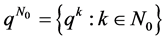with fixed are examples of time scales [2] [3] .

Definition 2.2. Assume is a function and. Then we define to be the number with the property that given any, there is a nighbourhood U (in T) of t such that

We call the delta (or Hilger) derivative of f at t.

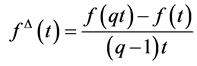is the usual Jakson derivative if.

Definition 2.3. If 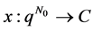is a function, then its q-Laplace transform is defined by

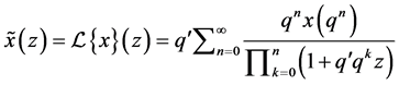(1)

for those values of, , for which this series converges, where.

Let us set

(2)

which is a polynomial in Z of degree. It is easily verified that the equations

(3)

and

(4)

hold, where. The numbers

where, belong to the real axis interval and tend to zero as. For any and, we set

and

so that is a closed domain of the complex plane C, whose points are in distance not less than from the set.

Lemma 2.4. For any,

(5)

Therefore, for an arbitrary number, there exists a positive integer such that

(6)

In particular,

(7)

Example 2.5. We find the q-Laplace transform of (k is a fixed number). We have in,

Example 2.6. We find the q-Laplace transform of the functions and .

We have (see [4] ),

On the other hand, we know that

with respect to

The q-Laplace transform of the functions and, would be

and

respectively.

Theorem 2.7. If the function satisfies the condition

(8)

where c and R are some positive constants, then the series in (1) converges uniformly with respect to z in the region and therefore its sum is an analytic (holomorphic) function in.

Proof. By Lemma 2.4, for the number R given in (8) we can choose an such that

Then for the general term of the series in (1), we have the estimate

Hence the proof is completed.

A larger class of functions for which the q-Laplace transform exists is the class of functions satisfying the condition

(9)

Theorem 2.8. For any, the series in (1) converges uniformly with respect to z in the region, and therefore its sum is an analytic function in.

Proof. By using the reverse (5), hence

and comparison test to get the desired result.

Theorem 2.9. (Initial Value and Final Value Theorem). We have the following:

a) If for some, then

(10)

b) If for all, then

(11)

Proof. Assume for some. It follows from (1) that

(12)

and

(13)

Hence

Multiplying, on both sides of the relation of (12) and by using equivalence relation, which yields (10). Note that we have taken a term-by-term limit due to the uniform convergence (Theorem 2.8) of the series in the region.

3. Convolutions

Definition 3.1. Let T be a time scale. We define the forward jump operator by

Definition 3.2. For a given function, its shift (or delay) is defined as the solution of the problem

(14)

Definition 3.3. For given functions, their convolution is defined by

(15)

where is the shift of f introduced in Definition 3.2 [4] .

Definition 3.4. For given functions, their convolution is defined by

with, where.

Theorem 3.5. (Convolution Theorem). Assume that, , and exist for a given. Then at the point z,

(16)

4. Concluding Remarks

1) We can see from Theorem 2.9(a) that no function has its q-Laplace transform equal to the constant function 1.

2) Finally, we note that most of the results concerning the Laplace transform on can be generalized appropriately to an arbitrary isolated time scale such that

Cite this paper

Maryam SimkhahAsil,ShahnazTaheri, (2016) q-Laplace Transform. Advances in Pure Mathematics,06,16-20. doi: 10.4236/apm.2016.61003

References

NOTES

^*Corresponding author.

References

- 1. Hilger, S. (1999) Special Function, Laplace and Fourier Transform on Measure Chains. Dynamic Systems and Applications, 8, 471-488.
- 2. Bohner, M. and Guseinov, G.Sh. (2007) The Convolution on Time Scales. Abstract and Applied Analysis, 2007, Article. ID: 58373.
http://dx.doi.org/10.1155/2007/58373 - 3. Michel, A.N., Hou, L. and Lio, D. (2007) Stability of Dynamical Systems Continuous, Discontinuous, and Discrete Systems. Boston, Basel, Berlin.
- 4. Bohner, M. and Guseinov, G.Sh. (2010) The h-Laplace and q-Laplace Transforms. Journal of Mathematical Analysis and Applications, 365, 75-92.
http://dx.doi.org/10.1016/j.jmaa.2009.09.061