ABSTRACT

Using the Picard iteration method and treating the involved integration by numerical quadrature formulas, we propose a numerical scheme for the second kind nonlinear Volterra integral equations. For enlarging the convergence region of the Picard iteration method, multistage algorithm is devised. We also introduce an algorithm for problems with some singularities at the limits of integration including fractional integral equations. Numerical tests verify the validity of the proposed schemes.

Keywords:

Volterra Integral Equation, Picard Iteration Method, Numerical Integration, Multistage Scheme

1. Introduction

The Volterra integral equations arise in many scientific and engineering fields such as the population dynamics, spread of epidemics, semi-conductor devices, vehicular traffic, the theory of optimal control, the kinetic theory of gases and economics [1] - [7] . The initial or boundary value problems for ordinary differential equations and some fractional differential equations can be equivalently expressed by the second-kind Volterra integral equation [6] - [9] .

In this work, we consider the general nonlinear Volterra integral equation of the second kind

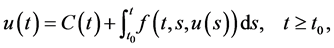(1)

where it permits weak singularity at the limits of integration.

The specific conditions under which a solution exists for the nonlinear Volterra integral equation are considered in [1] - [4] [7] . Many analytical and numerical methods have been proposed for solving this type of equations, such as the linearization and collocation method [10] - [14] , the trapezoidal numerical integration and implicit scheme method [15] , the implicit multistep collocation methods [16] , the reproducing kernel method [17] , the wavelet method [18] [19] , the Adomian decomposition method [6] [7] [20] and the methods by using function approximation [21] - [23] .

The Picard iteration method, or the successive approximations method, is a direct and convenient technique for the resolution of differential equations. This method solves any problem by finding successive approximations to the solution by starting with the zeroth approximation. The symbolic computation applied to the Picard iteration is considered in [24] [25] , and the Picard iteration can be used to generate the Taylor series solution for an ordinary differential equation [25] .

In this work, we concern on the numerical Picard iteration methods for nonlinear Volterra integral Equation (1). By using the proposed methods, we treat the involved integrals numerically and enlarge the effective region of convergence of the Picard iteration. The rest of the paper is organized as follows. In Section 2, the scheme in a single interval is considered, and the validity of the method is verified by some numerical tests. Basing on the scheme proposed in Section 2, we devise a multistage algorithm in Section 3 for enlarging the convergence region. In Section 4, an algorithm is introduced for problems with some singularity. To show the effectiveness of the proposed algorithms, we perform some numerical results.

2. Numerical Picard Iteration Method for Integral Equations

The Picard iteration scheme for the considered Equation (1) reads [7] [26]

(2)

(3)

The Picard iteration scheme has been applied in almost each textbook on differential equations to mainly prove the existence and uniqueness of solutions. It is direct and easily learned for numerical calculation.

Assume the recursion scheme is convergent for. Denote

At, (3) becomes

(4)

Treating the integral involved in (4) by numerical quadrature formulas, we have the numerical Picard iteration scheme for (1) over

(5)

(6)

where and are the corresponding weights. Considering the compound trapezoidal formula in (6), the weights are

Numerical results are given to validate the proposed scheme. Let us start with an example in which the inte- grand 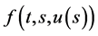is independent with t.

Example 1 Consider the initial value problem (IVP) for the nonlinear differential equation

This IVP has the exact solution

The equivalent integral equation of the IVP is

Denote the result after iterations when discretization parameter N is taken. Take T = 10, N = 20. Figure 1(a) and Figure 1(b) show the results of the first 5 iterations and the errors at T for each iteration respectively. It’s shown in the figure that, the iterative solution converges exponentially respect to iteration num- ber n.

The relative errors are larger than when N = 20. For higher accuracy, more nodes in

numerical integration are needed. For each fixed N, iterations stop when. Errors for are plotted in Figure 2(a). Especially at T, we report the dependence of the error on n and N in Figure 2(b) and Figure 2(c), respectively. The figures show that the errors increase respect to t and decrease respect to n exponentially, and decrease respect to N at an order about

.

Next we give an example with t-dependent integrand.

Example 2 Consider the pendulum equation

(7)

The exact solution can be expressed in terms of the Jacobi elliptic function

Integrating the differential equation in (7) yields

Take,. Similar behavior of errors as in Figure 1 can be observed from Figure 3 which shows

the results of the first 5 iterations and the errors at T for each iteration. It confirms the validity of the scheme (5), (6) for equations with general integrand f.

What’s different from Example 1 is that, at T, the results of the second and the third iterations are even worse than the first one. However, it can be noticed that, in the interval closer to t = 0, for example, the errors decrease as n increases all the same. So the underlying numerical iteration method can be viewed as a point-by- point correction process.

3. Multistage Scheme

It’s well-known that the convergence of the Picard iteration is constrained in some interval. Then how can we get the numerical solution to the integral Equation (1) when t is outside the interval of convergence? We will take advantage of the multistage method and design a scheme by which the considered problem can be solved interval by interval. For example, the Equation (1) is considered on, however, assume that the single- stage-scheme designed in the previous section is convergent only on, where t₁ < T. For achieving the numerical result at T, we can regard the problem on as a new one, in which we take the numerical result at as the initial value. Now we begin to design the multistage scheme in detail.

Denote the time interval considered for (1) by. For a given positive integer K, we break I into K disjoint subintervals such that,

where. For, take uniformly distributed nodes on satisfy- ing

(8)

Suppose the equation has been solved on, namely, the first subintervals. For (), denote the times of iteration by and the iterative solutions by, where.

Now we consider the solution on. Taking in (1),

we have for,

(9)

the right hand side of which will be analyzed below.

・ An approximation of the first term has been gotten in previous resolution.

・ The second part, with the approximations of on nodes in having been gained, can also be ap- proximated

where the corresponding weights for numerical integration on are

(10)

・ can be calculated directly.

Denoting

(11)

(9) leads to a new equation, which is similar to the considered problem (1),

namely,

(12)

Using (5), (6) over, numerical solution to (12) can be obtained.

We conclude the previous analysis as an algorithm.

Algorithm 1 Choose the algorithm’s parameters: number of subintervals, set of nodes and discretization parameters.

Step 1. For, generate

- the uniformly distributed nodes and corresponding weights on according to (8) and (10)

- the weights for numerical integration on ,

Step 2. For k = 1, solve (12). Note that the first term of. So solving (12) for k = 1 is equivalent to solving the original Equation (1) for. Use (5), (6) with instead of.

Step 3. Recursively solve (12) for using a similar scheme to (2) as follows:

- Calculate by (11).

- The initial value of iteration:

- For, and

Here, we perform a numerical test to examine the effectiveness of Algorithm 1 and compare it with the scheme in single interval (2).

Example 3 Consider the Lane-Emden equation

The exact solution is

The equivalent integral form of the Lane?Emden equation is [20]

First, taking T = 4, , we solve the current problem by (5), (6). The numerical solutions of the first 5 iterations and the errors at T are shown in Figure 4 from which the convergence can be observed. Unfortunately, the scheme is not convergent for T = 6.

Consider the underlying problem for larger T by Algorithm 1. The time interval is uniformly divided into K subintervals, in which the same discretization parameter, denoted by N, is taken. Take and. For each N, iterations on () stop when

(13)

where denotes the result after n iterations when discretization parameters N and K are taken. Errors and convergence rates respect to N at t = 12 are reported in Table 1, from which one can see that the underlying scheme is of order.

In fact, from the errors reported in the table, the convergence order can also be obtained. So the scheme is of order. Errors for K = 3 and N = 10, 20, 30, 40 are plotted in Figure 5(a). The validity of Algorithm 1 is numerically confirmed.

It’s an interesting phenomenon observed from Table 1 that almost the same results are obtained for same NK. For example, when NK = 120, the errors are all. This may be because “enough” iteration numbers are taken for all subintervals in the sense of (13). Setting the maximal iteration number allowed for each sub- interval to 3 and taking NK = 120, we recalculate the current example up to T = 12 for K = 3, 4, 5, 6, 8, 10, 12, 15. The errors at T are presented in Figure 5(b) which shows the decrement of the errors respect to K.

4. Problem with Singular Integrand

In recent years, the fractional differential or integral equations are much involved. In fact, fractional integral is a class of integration with weak singular kernel. So many fractional differential and integral equations can be equivalently expressed by the singular Volterra integral equation of the second kind. Let us consider such an integral equation with some singularity.

Example 4 Consider the singular Volterra integral equation [14]

The exact solution is. Note that in the integrand there has, which is infinity at. Insuch case, the numerical scheme (5), (6) and corresponding multistage scheme (Algorithm 1) are not valid any more.

A simple idea is to avoid the value of the integrand at s = t in the numerical integration, so an alternative is to

integrate with compound rectangular formula. The only things we need to do are changing the nodes of numerical integration and generating approximations for the values of on these points since only the values on the

nodes have been gained.

For, denote the midpoint of () and the corresponding weight by

(14)

Denote

(15)

in which

Thus, (12) becomes

(16)

We present the following algorithm.

Algorithm 2 Choose the algorithm’s parameters: number of subintervals, set of nodes and discretization parameters.

Step 1. For, generate

- the nodes on according to (8).

- the integral nodes and weights on according to (14).

- the weights for numerical integration on ,

Step 2. Solve (16) for k = 1. As in Algorithm 1, since, it is equivalent to solving (1) for. Detail algorithm reads:

- For, calculate and get the initial value of iteration:.

- For, and

where.

Step 3. Recursively solve (16) for as follows:

- For, calculate by (15) and get the initial value of iteration:

- For, and

where.

Now, we come back to Example 4. Taking to subdivide the time interval and N = 5, 10, 20, 40. Figure 6 presents the dependence of the error on for each N and that on N at t = 1. The results verify the validity of Algorithm 2 in solving problems with some singularity at the limits of integration. However, the method is of order about only for this example.

Remark 1. Algorithm 2 is devised not especially for singular problems. It’s also valid for regular problems. For instance, we recalculate Example 1 with K = 2 and N = 5, 10, 20, 40, 80, 160. Errors and convergence rates respect to N are reported in Table 2, from which we can find the order is.

5. Conclusions

In this work, Picard iteration methods with numerical integration are devised for the second kind nonlinear Volterra integral equations. The Picard iteration method solves the considered nonlinear equation explicitly, while the multistage scheme solves it interval by interval and enlarges the convergence region of the Picard iteration method. Numerical results validate the proposed schemes and algorithms and reveal that the schemes are of order for regular problems.

What should be noticed is that the errors reported in the numerical results decrease exponentially respect to times of iteration n (for example, through simple calculation, we can observe from Figure 3(b) and Figure 4(b) that the convergence rates are about for Examples 2 and 3) and are of order respect to discretization parameter NK. Future work may concern on enhancing the rate of convergence respect to NK.

Acknowledgements

This work was supported by the Natural Science Foundation of Shanghai (No. 14ZR1440800) and the Innovation Program of the Shanghai Municipal Education Commission (No. 14ZZ161).

Cite this paper

Lian Chen,Junsheng Duan, (2015) Multistage Numerical Picard Iteration Methods for Nonlinear Volterra Integral Equations of the Second Kind. Advances in Pure Mathematics,05,672-682. doi: 10.4236/apm.2015.511061

References

NOTES

^*Corresponding author.

References

- 1. Davis, H.T. (1962) Introduction to Nonlinear Differential and Integral Equations. Dover, Publications, New York.
- 2. Jerri, A. (1999) Introduction to Integral Equations with Applications. Wiley, New York.
- 3. Linz, P. (1985) Analytical and Numerical Methods for Volterra Equations. SIAM, Philadelphia.
http://dx.doi.org/10.1137/1.9781611970852 - 4. Miller, R.K. (1967) Nonlinear Volterra Integral Equations. W. A. Benjamin, Menlo Park.
- 5. Wazwaz, A.M. (1997) A First Course in Integral Equations. World Scientific, Singapore City.
http://dx.doi.org/10.1142/3444 - 6. Wazwaz, A.M. (2009) Partial Differential Equations and Solitary Waves Theory. Higher Education, Beijing, and Springer, Berlin.
http://dx.doi.org/10.1007/978-3-642-00251-9 - 7. Wazwaz, A.M. (2011) Linear and Nonlinear Integral Equations: Methods and Applications. Higher Education, Beijing, and Springer, Berlin.
http://dx.doi.org/10.1007/978-3-642-21449-3 - 8. Duan, J.S. and Rach, R. (2011) A New Modification of the Adomian Decomposition Method for Solving Boundary Value Problems for Higher Order Nonlinear Differential Equations. Applied Mathematics and Computation, 218, 4090-4118.
http://dx.doi.org/10.1016/j.amc.2011.09.037 - 9. Daftardar-Gejji, V. and Jafari, H. (2006) An Iterative Method for Solving Nonlinear Functional Equations. Journal of Mathematical Analysis and Application, 316, 753-763.
http://dx.doi.org/10.1016/j.jmaa.2005.05.009 - 10. Maleknejad, K. and Najafi, E. (2011) Numerical Solution of Nonlinear Volterra Integral Equations Using the Idea of Quasilinearization. Communications in Nonlinear Science and Numerical Simulation, 16, 93-100.
http://dx.doi.org/10.1016/j.cnsns.2010.04.002 - 11. Brunner, H. (2004) Collocation Methods for Volterra Integral and Related Functional Equations. Cambridge University Press, Cambridge.
http://dx.doi.org/10.1017/CBO9780511543234 - 12. Brunner, H., Pedas, A. and Vainikko, G. (2001) A Spline Collocation Method for Linear Volterra Integro-Differential Equations with Weakly Singular Kernels. BIT Numerical Mathematics, 41, 891-900.
http://dx.doi.org/10.1023/A:1021920724315 - 13. Brunner, H., Pedas, A. and Vainikko, G. (2001) Piecewise Polynomial Collocation Method for Linear Volterra Integro-Differential Equations with Weakly Singular Kernels. SIAM Journal on Numerical Analysis, 39, 957-982.
http://dx.doi.org/10.1137/S0036142900376560 - 14. Te Riele, H.J.J. (1982) Collocation Methods for Weakly Singular Second-Kind Volterra Integral Equations with Non-Smooth Solution. IMA Journal of Numerical Analysis, 2, 437-449.
http://dx.doi.org/10.1093/imanum/2.4.437 - 15. Atkinson, K.E., Han, W. and Stewart, D. (2009) Numerical Solution of Ordinary Differential Equations. John Wiley & Sons, Hoboken.
http://dx.doi.org/10.1002/9781118164495 - 16. Fazeli, S., Hojjati, G. and Shahmorad, S. (2012) Super Implicit Multistep Collocation Methods for Nonlinear Volterra Integral Equations. Mathematical and Computer Modelling, 55, 590-607.
http://dx.doi.org/10.1016/j.mcm.2011.08.034 - 17. Ketabchi, R., Mokhtari, R. and Babolian, E. (2015) Some Error Estimates for Solving Volterra Integral Equations by Using the Reproducing Kernel Method. Journal of Computational and Applied Mathematics, 273, 245-250.
http://dx.doi.org/10.1016/j.cam.2014.06.016 - 18. Saberi-Nadjafi, J., Mehrabinezhad, M. and Akbari, H. (2012) Solving Volterra Integral Equations of the Second Kind by Wavelet-Galerkin Scheme. Computers & Mathematics with Applications, 63, 1536-1547.
http://dx.doi.org/10.1016/j.camwa.2012.03.043 - 19. Yousefi, S.A. (2006) Numerical Solution of Abel’s Integral Equation by Using Legendre Wavelets. Applied Mathematics and Computation, 175, 574-580.
http://dx.doi.org/10.1016/j.amc.2005.07.032 - 20. Wazwaz, A.M., Rach, R. and Duan J.S. (2013) Adomian Decomposition Method for Solving the Volterra Integral Form of the Lane-Emden Equations with Initial Values and Boundary Conditions. Applied Mathematics and Computation, 219, 5004-5019.
http://dx.doi.org/10.1016/j.amc.2012.11.012 - 21. Costarelli, D. and Spigler, R. (2013) Solving Volterra Integral Equations of the 2nd Kind by Sigmoidal Functions Approximations. Journal of Integral Equations and Applications, 25, 193-222.
http://dx.doi.org/10.1216/JIE-2013-25-2-193 - 22. Costarelli, D. and Spigler, R. (2014) A Collocation Method for Solving Nonlinear Volterra Integro-Differential Equations of the Neutral Type by Sigmoidal Functions. Journal of Integral Equations and Applications, 26, 15-52.
http://dx.doi.org/10.1216/JIE-2014-26-1-15 - 23. Maleknejad, K., Hashemizadeh, E. and Ezzati, R. (2011) A New Approach to the Numerical Solution of Volterra Integral Equations by Using Bernstein’s Approximation. Communications in Nonlinear Science and Numerical Simulation, 16, 647-655.
http://dx.doi.org/10.1016/j.cnsns.2010.05.006 - 24. Mathews, J. (1989) Symbolic Computational Algebra Applied to Picard Iteration. Mathematics and Computer Education, 23, 117-122.
- 25. Parker, G.E. and Sochacki, J.S. (1996) Implementing the Picard Iteration. Neural, Parallel and Scientific Computations, 4, 97-112.
- 26. Bailey, P.B., Shampine, L.F. and Waltman, P.E. (1968) Nonlinear Two Point Boundary Value Problems. Academic, New York/London.