Advances in Pure Mathematics
Vol.3 No.9(2013), Article ID:40882,5 pages DOI:10.4236/apm.2013.39095
A New Application of the Flux Approximation Method on Hyperbolic Conservation Systems
1Department of Mathematics, Hangzhou Normal University, Hangzhou, China
2Departamento de Matemáticas, Universidad Nacional de Colombia, Bogotá, Colombia
Email: *deyinzheng@hznu.edu.cn
Copyright © 2013 Yunguang Lu et al. This is an open access article distributed under the Creative Commons Attribution License, which permits unrestricted use, distribution, and reproduction in any medium, provided the original work is properly cited. In accordance of the Creative Commons Attribution License all Copyrights © 2013 are reserved for SCIRP and the owner of the intellectual property Yunguang Lu et al. All Copyright © 2013 are guarded by law and by SCIRP as a guardian.
Received November 14, 2013; revised December 8, 2013; accepted December 15, 2013
Keywords: Flux Approximation; Viscosity Approximation; Hyperbolic Conservation Laws; Weak Solutions; Compensated Compactness Method
ABSTRACT
In this paper, we first summarize several applications of the flux approximation method on hyperbolic conservation systems. Then, we introduce two hyperbolic conservation systems (2.1) and (2.2) of Temple’s type, and prove that the global weak solutions of each system could be obtained by the limit of the linear combination of two systems.
1. Introduction
It is well known that no classical solution exists for the following initial value problem
 (1.1)
(1.1)
with bounded measurable initial data
 (1.2)
(1.2)
where  is the unknown vector function standing for the density of physical quantities and
  is a given vector function denoting the conservative term. These equations are commonly called conservation laws.
Since, in general, the discontinuity or the shock waves will appear in the solution to the Cauchy problem (1.1)- (1.2), there are two standard methods to obtain a weak solution or a generalized solution  for given hyperbolic conservation laws. One is to construct a sequence of smooth functions to approximate
 . For example, to add a small parabolic perturbation term to the right-hand side of (1.1):
 (1.3)
(1.3)
where 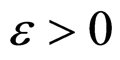 is a constant. For each fixed
 , we have a classical solution
 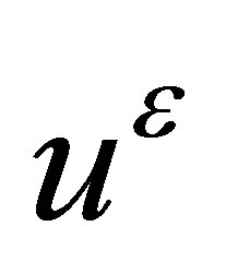 of (1.3)-(1.2), then we try to prove that the limit
  of
of  as
as  goes to zero is the solution of (1.1)-(1.2), where the compactness could be obtained by the compensated compactness arguments [1,2] when the functions have only the uniform boundedness in a suitable Banach space or the technique given in [3] when the functions are of total bounded variation estimates; another is the finite difference method [4]. We construct a sequence of simple functions by choosing a suitable difference scheme which is based on the given hyperbolic conservation laws and then prove the compactness of the sequence of functions. Normally, in the second method, we know that the sequence of simple functions is of total bounded variation estimates.
However, the third front tracking method [5], here we just call it the flux approximation method, is also used in many different cases.
In [6], Dafermos first introduced this method to the scalar conservation law
 (1.4)
(1.4)
where  is a scalar function, and
 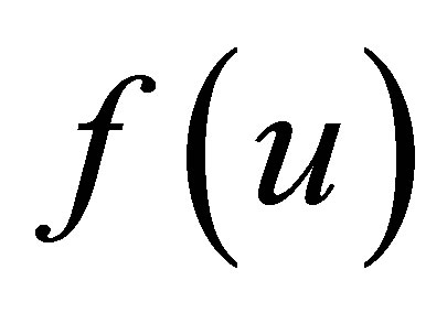 is a locally Lipschitz continuous function. He constructed a sequence of piecewise linear functions
 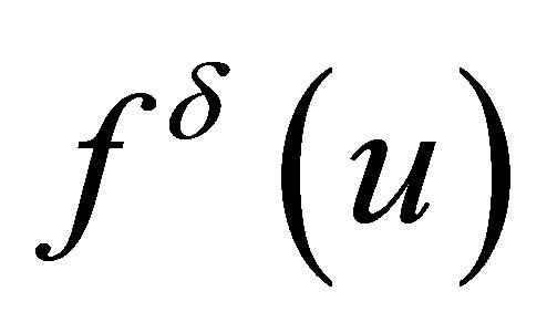 and a sequence of step functions
  to approximate
  and the initial date
 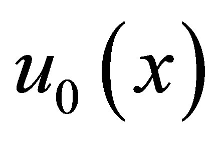 respectively. Let the solutions of the following Cauchy problem be
 :
:
 (1.5)
(1.5)
with the initial data
 (1.6)
(1.6)
For each fixed , since the simplicity of the flux function
  and the initial date
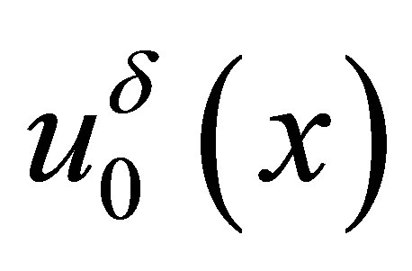 , the sequence of solutions
 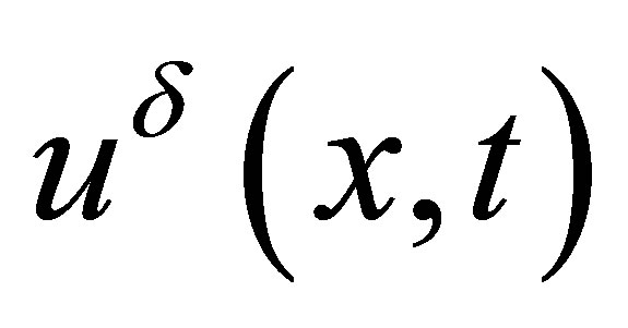 can be easily obtained first. Then by using the standard compactness argument by Oleinik, the convergence of
  can be proved as
  goes to zero.
Later, the above idea was used to study the existence of Riemann solutions for some special systems of two equations. For example, in [7], the author first studied the Riemann solution for the Cauchy problem of the following system
 (1.7)
(1.7)
with initial data
 (1.8)
(1.8)
The more details about the Front Tracking method for systems of hyperbolic conservation laws can be found in the books [5,8] and the references cited therein.
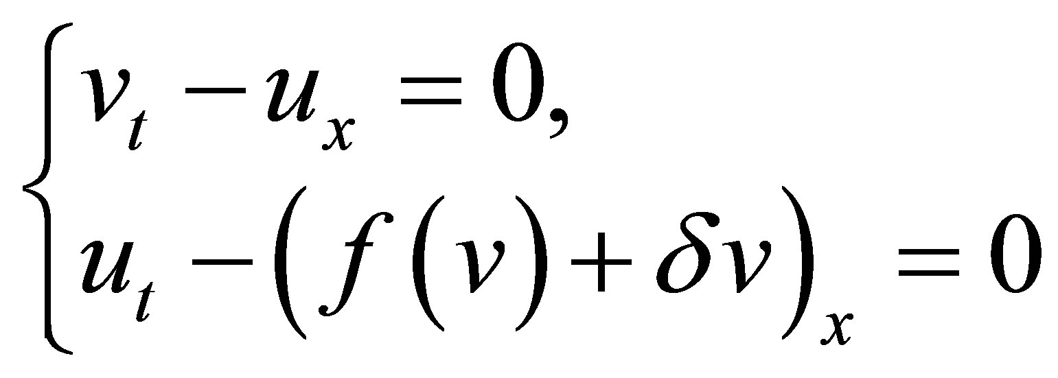
In [9], Keyfitz introduced a different way to approximate the nonlinear flux function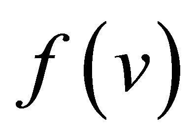 . Consider the Cauchy problem
 (1.9)
(1.9)
with the Riemann initial data, where 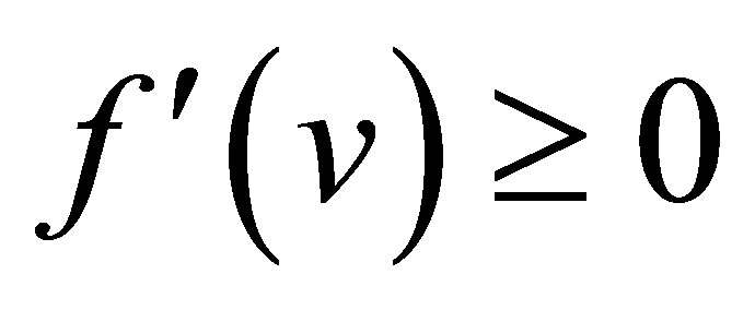 since the system is hyperbolic or
 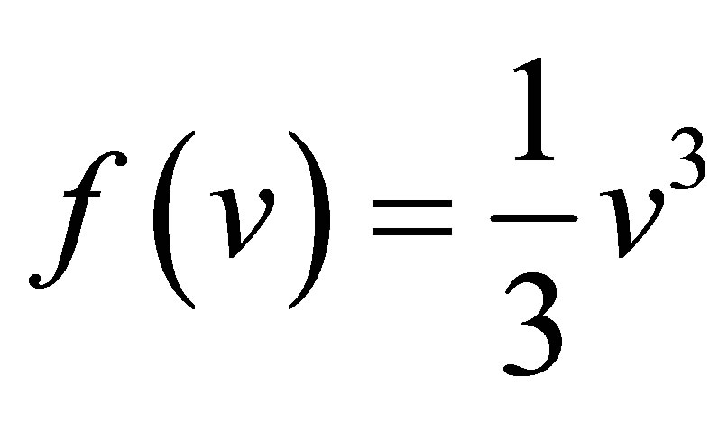 as required in
[9]. For each fixed , System (1.9) is strictly hyperbolic and Riemann solution
  could be easily obtained. Then a Riemann solution of system (1.7) follows since it is the limit of
  as
as  goes to zero.
The method of flux approximation was applied by the first author of this paper to study the existence of weak solutions [10,11], the existence of global Lipschitz solutions [12], 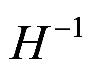 compactness for weak entropy-entropy flux pairs of the isentropic gas dynamics [11],
 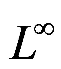 estimate for isentropic gas dynamics with a superline source [13], the global
  solutions of Aw-Rascle traffic flow model [14] (or the nonsymmetric systems of Keyfitz-Kranzer type) with negative adiabatic exponent and so on, which we shall introduce below. A new application of this method related to the LeRoux system is introduced in Theorem 1, Section 2.
2. A New Application of Flux Approximation Method
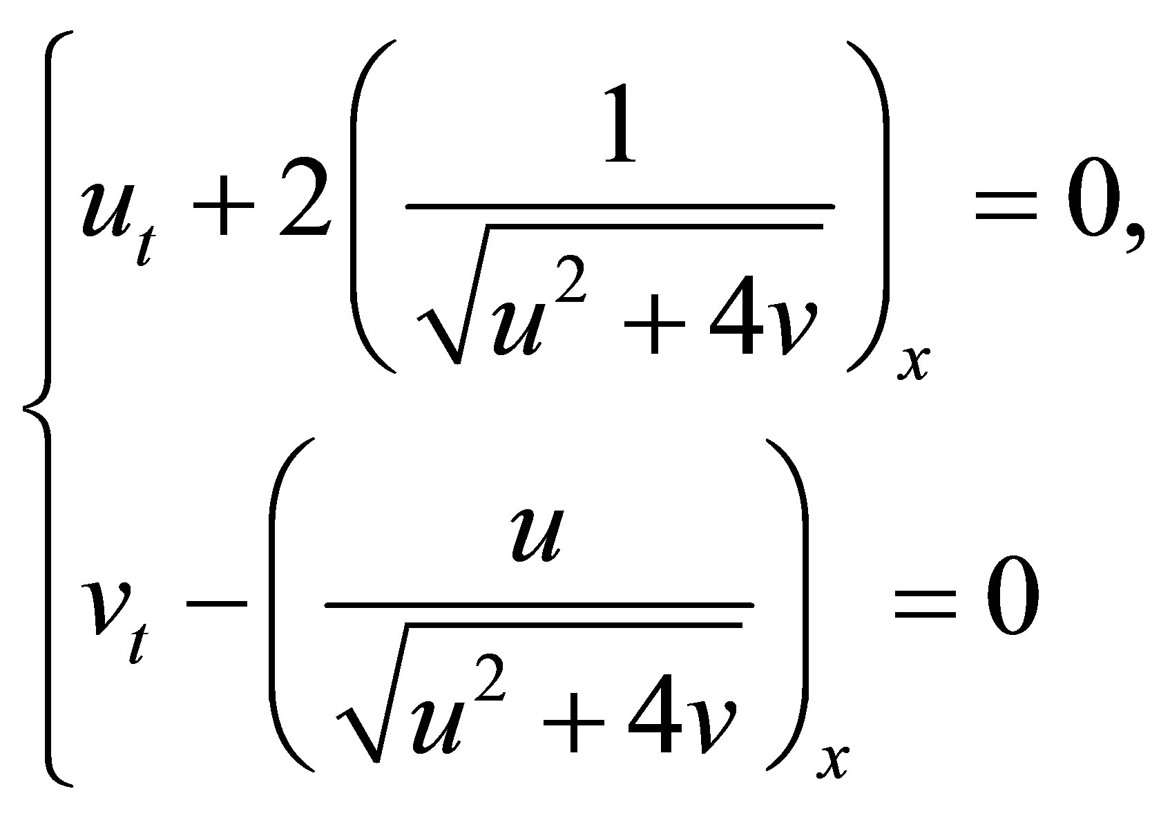
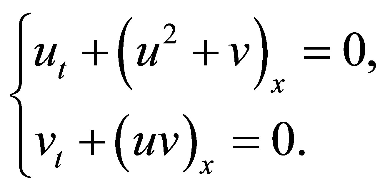
In this section, we introduce a new application of the flux approximation method. We found two hyperbolic conservation systems of Temple’s type [15], and the global weak solution of each system could be obtained by the limit of the linear combination of two systems.
Consider the hyperbolic systems
 (2.1)
(2.1)
and
 (2.2)
(2.2)
By simple calculations, two eigenvalues of system (2.1) are
 (2.3)
(2.3)
where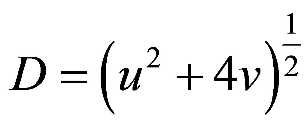 , with corresponding right eigenvectors
 (2.4)
(2.4)
and
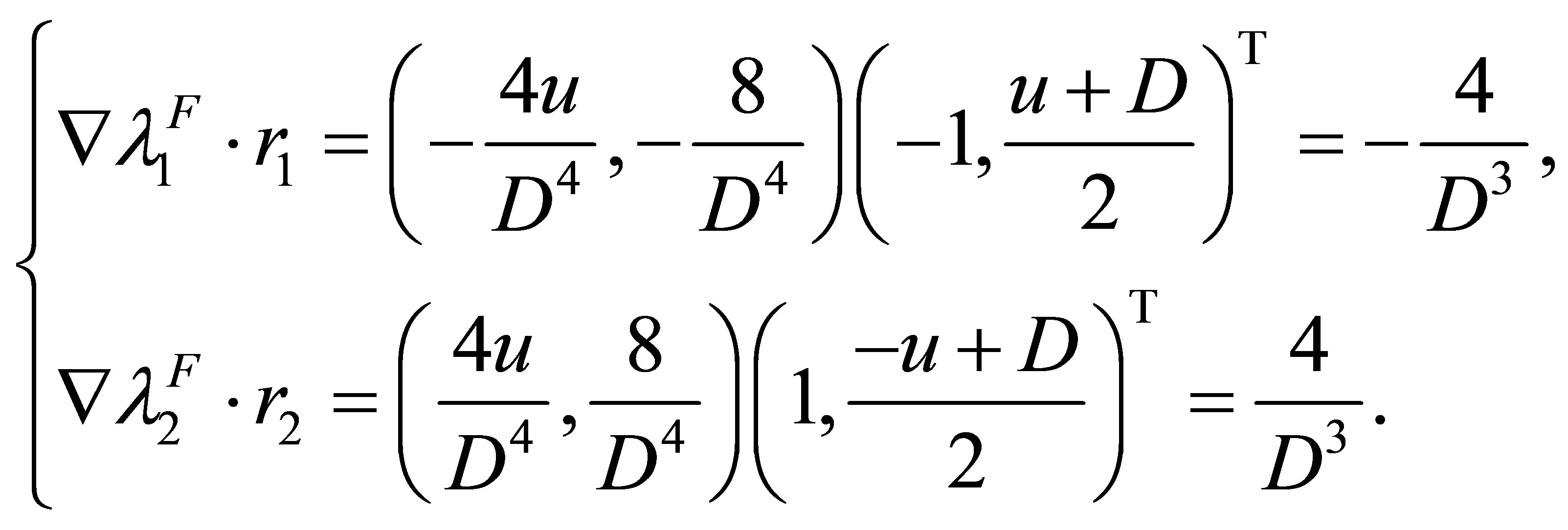 (2.5)
(2.5)
The Riemann invariants of (2.1) are
 (2.6)
(2.6)
Thus, the curves  are straight lines on the
  -plane.
Similarly, two eigenvalues of system (2.2) are
 (2.7)
(2.7)
with the corresponding right eigenvectors (2.4) and
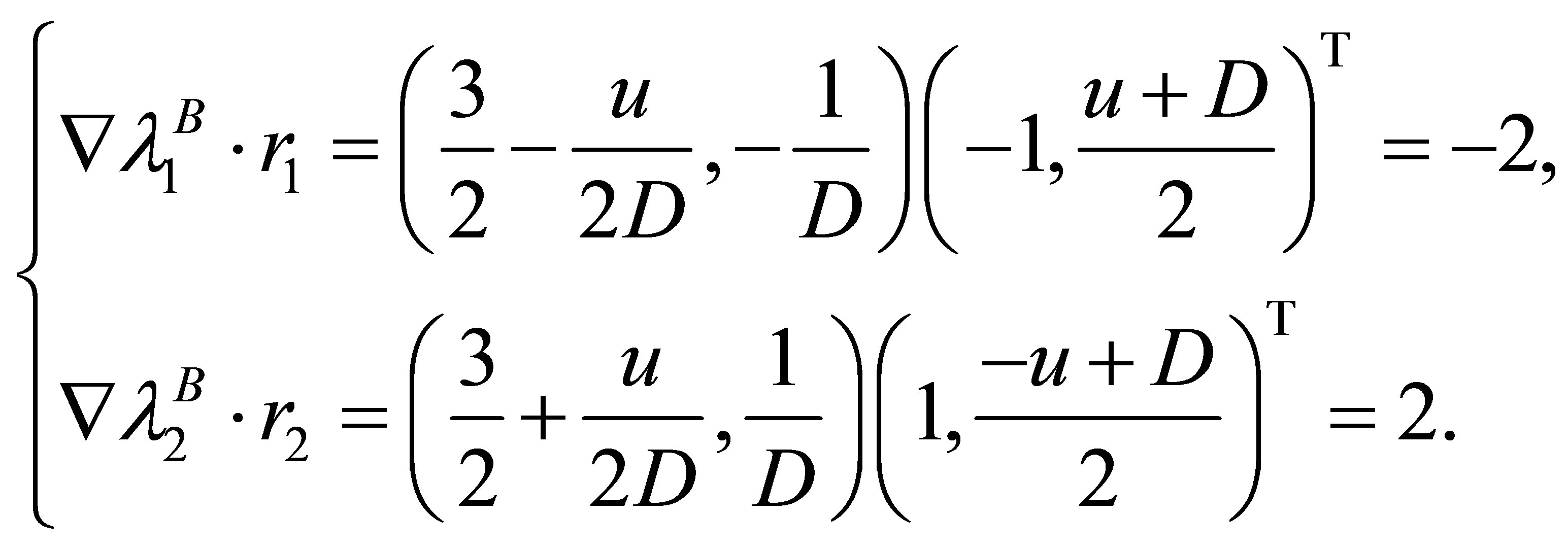 (2.8)
(2.8)
The Riemann invariants of (2.2) are also given by (2.6)
Therefore if we consider the bounded solution in the region: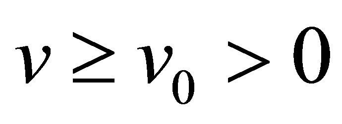 , it follows from (2.5) (or (2.8)) that both characteristic fields of system (2.1) (or system (2.2)) are genuinely nonlinear in the sense of Lax [16].
Now we prove that both systems (2.1) and (2.2) have the same entropies.
Let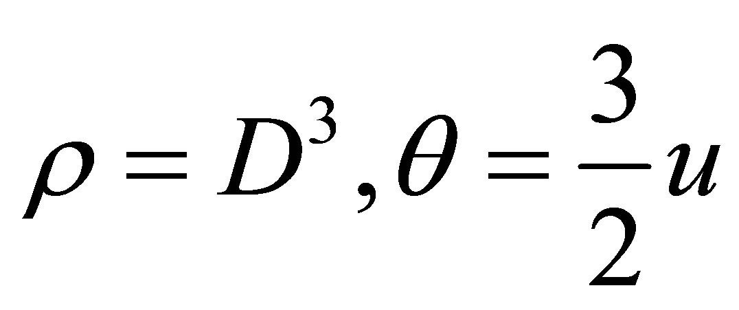 . Then for smooth solutions, (2.2) is equivalent to the following system:
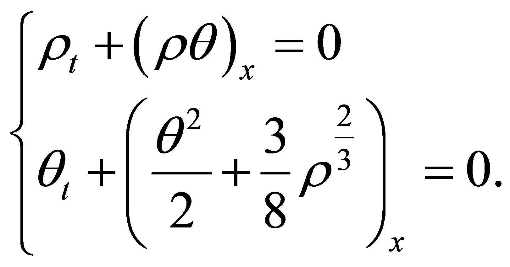 (2.9)
(2.9)
Considering the entropy-entropy flux pair 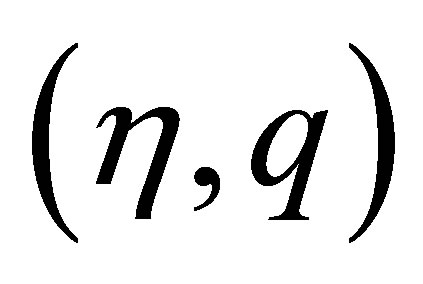 of system (2.2) as functions of variables
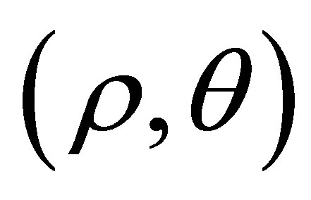 , we have
 (2.10)
Eliminating the  from (2.10), we have
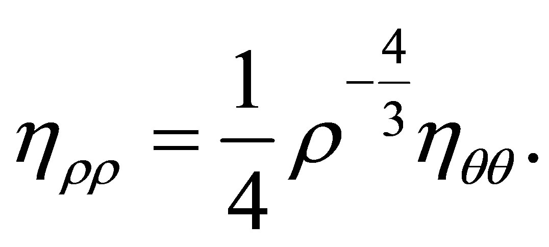 (2.11)
Similarly, for smooth solutions, (2.1) is equivalent to the following system:
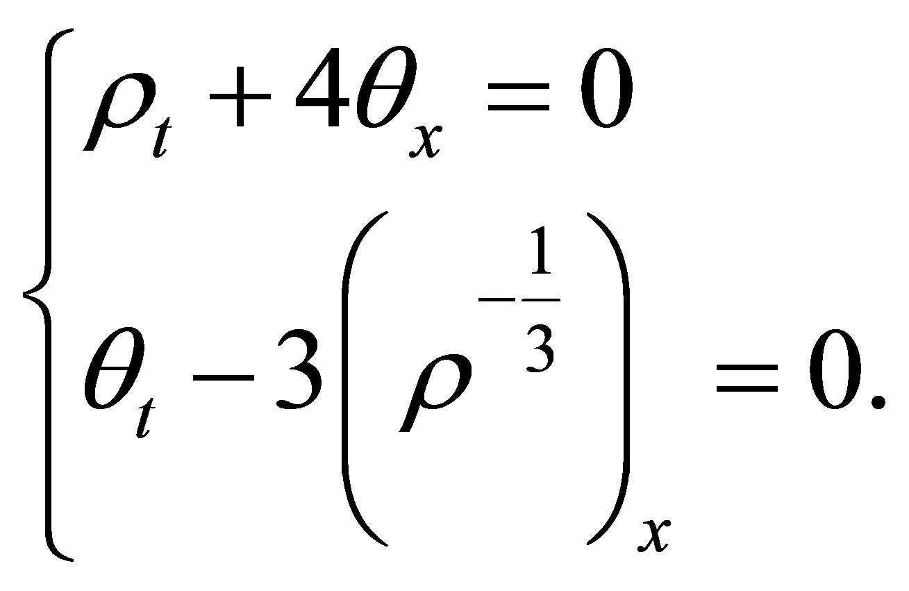 (2.12)
For the entropy-entropy flux pair  of system (2.1), we have
 (2.13)
Eliminating the 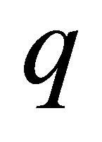 from (2.13), we have also the same entropy Equation (2.11).
Using the compensated compactness arguments, we may easily obtain the global existence of weak solutions for the Cauchy problem of system (2.2) in the upper  -plane
 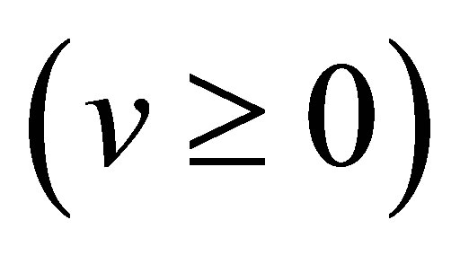 or system (2.1) in the region
  for a suitable constant
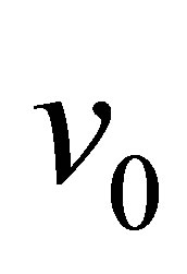 , which could be guaranteed since the curves
  are straight lines, where
  are four suitable constants. The details could be found in Chapter 7 of [17] or the original paper by Diperna [18].
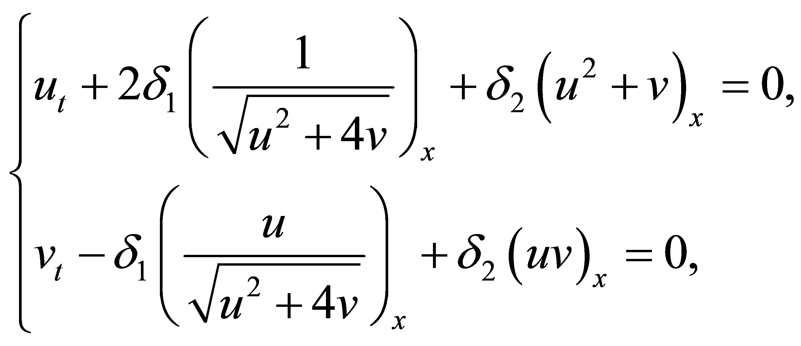
Now we consider the linear combination of systems (2.1) and (2.2):
 (2.14)
where 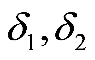 are two positive flux approximation perturbations.
The eigenvalues of system (2.14) are solutions of the following characteristic equation:
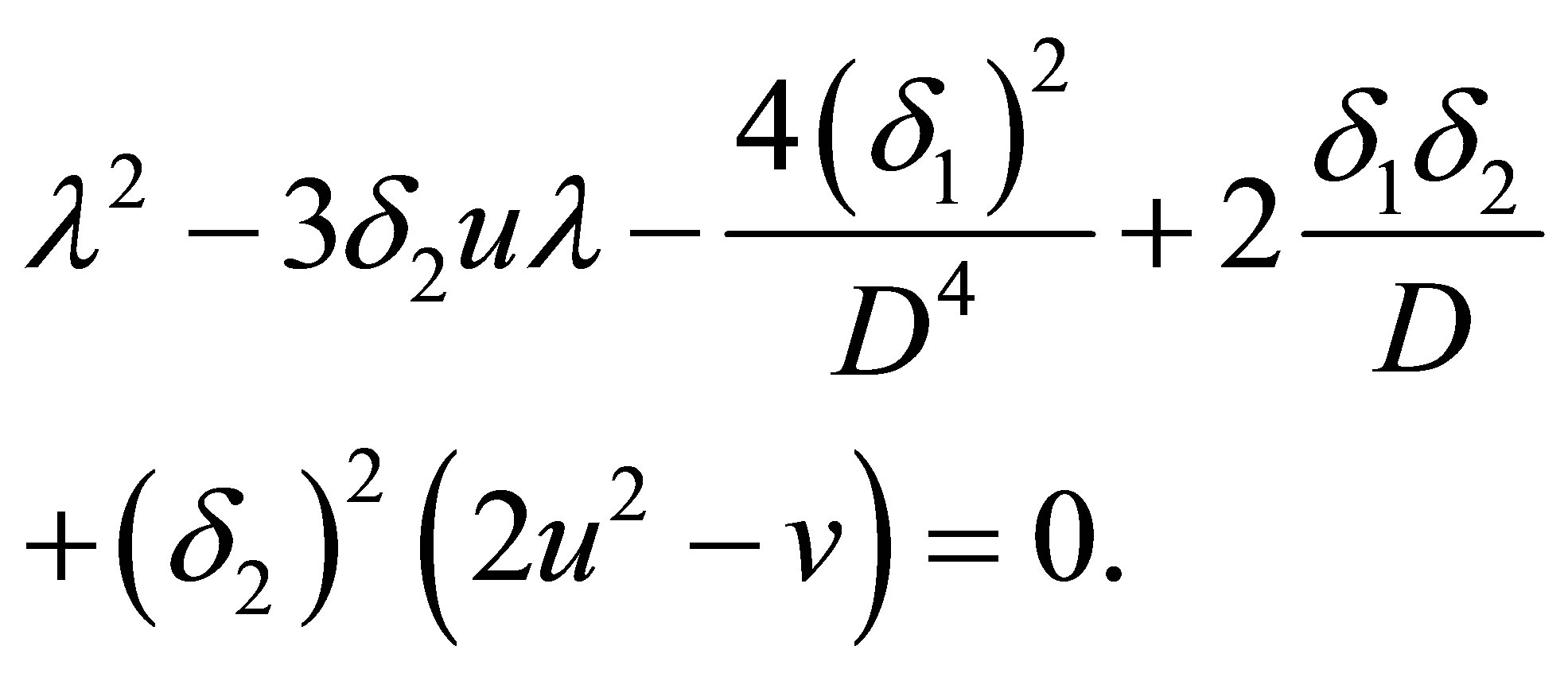 (2.15)
Two roots of Equation (2.15) are
 (2.16)
with the corresponding right eigenvectors (2.4) and the Riemann invariants (2.6). Moreover,
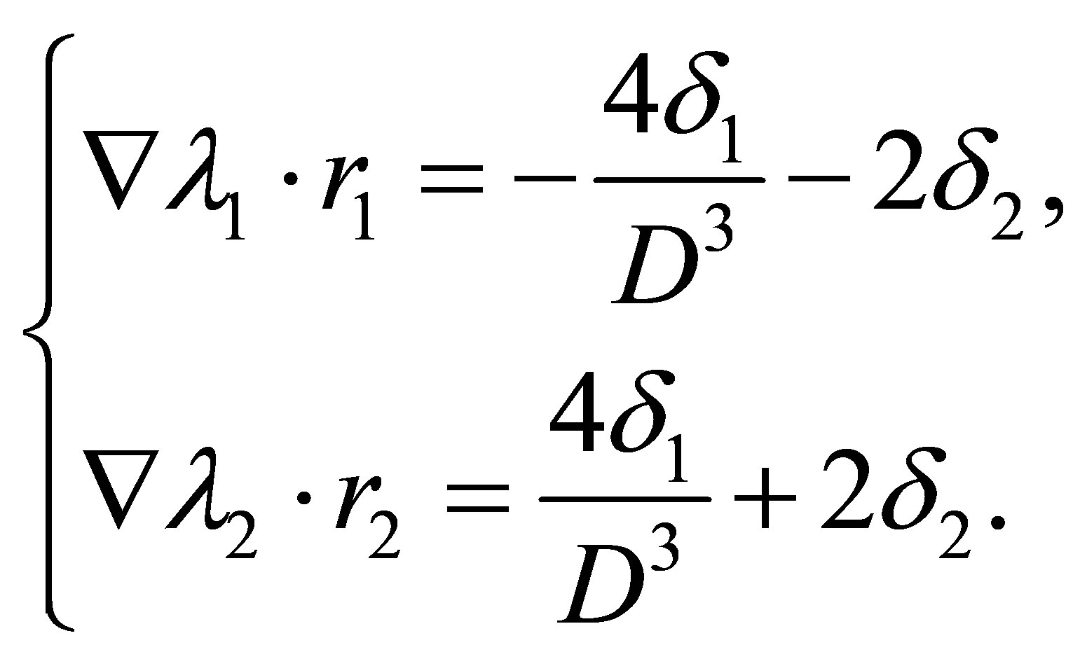 (2.17)
Therefore both characteristic fields of system (2.14) are genuinely nonlinear in the region: .
.
Now we consider the Cauchy problem of system (2.14) with initial data
 (2.18)
and have the main results in the following theorem
Theorem 1. Suppose the initial data  be bounded measurable and
  for a suitable constant
 . Then for any fixed
 , the global weak solution
  of the Cauchy problem (2.14) and (2.18) exists. Moreover, for fixed
 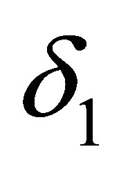 (or
(or ), there exists a subsequence
 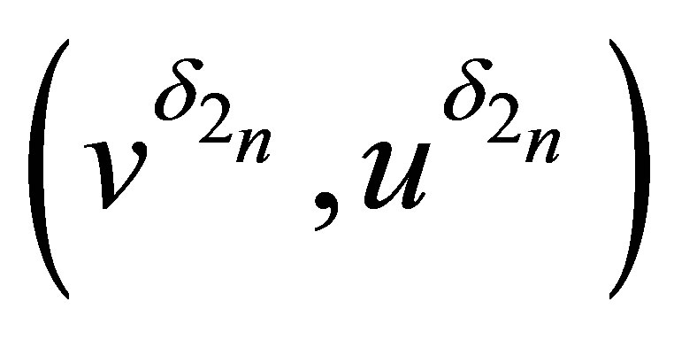 (or
(or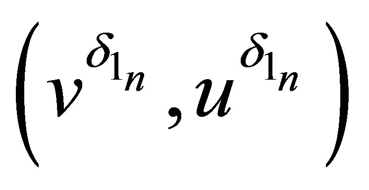 ) of
) of , which piontwisely converges, as
 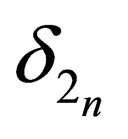 (or
(or ) goes to zero, to the solution of the Cauchy problem of system (2.1) (or (2.2)) with the initial data (2.18).
The proof of Theorem 1: The proof of Theorem 1 can be obtained by the standard vanishing artificial viscosity method coupled with the compensated compactness argument and the famous framework of DiPerna [18] for strictly hyperbolic, genuinely nonlinear systems of two equations. We add the viscosity terms to the right hand side of (2.14) and consider the following parabolic system
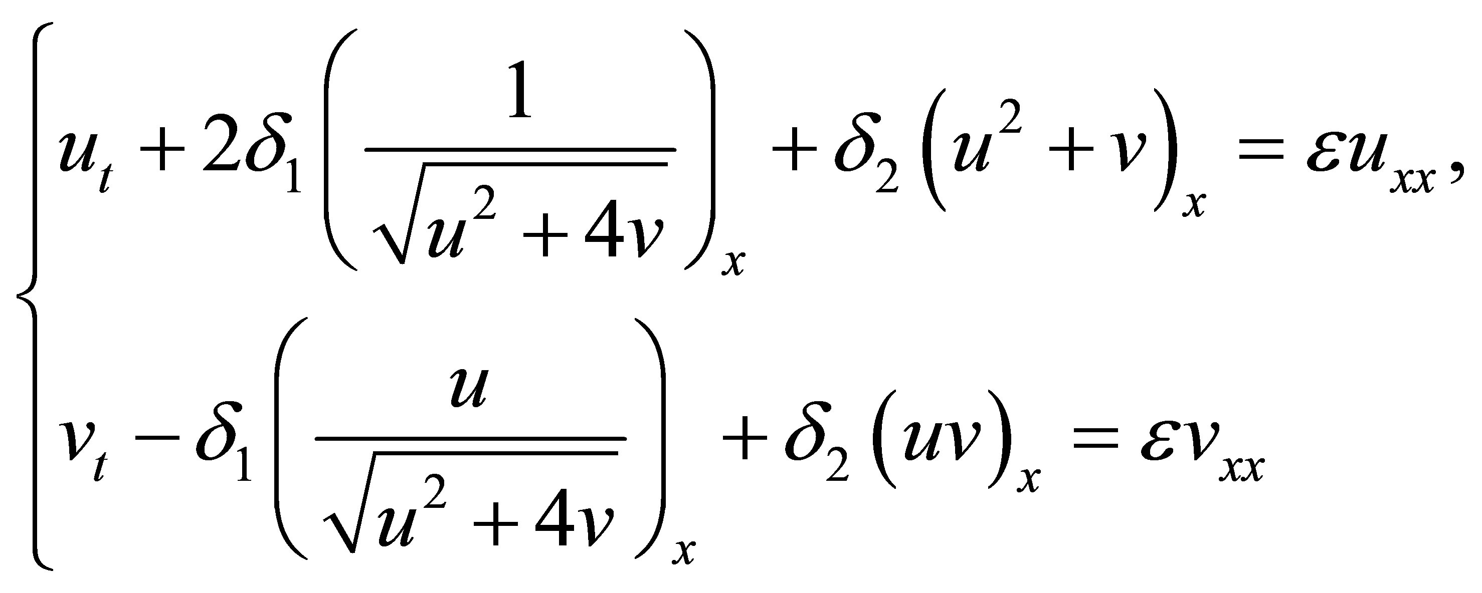 (2.19)
with the initial data (2.18). According to the calculations given in (2.3) and (2.7), we know that the two eigenvalues of system (2.14) are
 (2.20)
with the corresponding right eigenvectors (2.4) and the Riemann invariants (2.6).
For any constant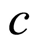 , the curves
 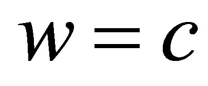 or
or  is a straight line on the
 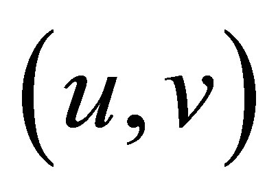 -plane, then we may choose suitable constants
  such that
  forms a bounded invariant region. Moreover, in this region,
 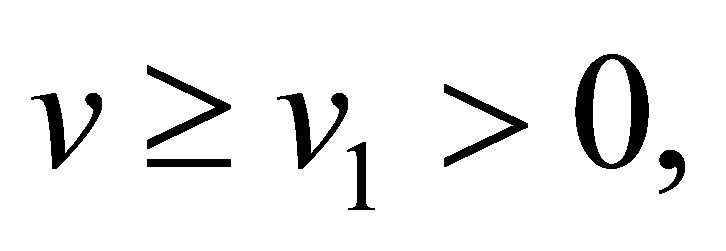 for a suitable constant
 . Since system (2.14) is strictly hyperbolic and genuinely nonlinear, and the viscosity solutions
  of system (2.19) are uniformly bounded, then the famous compactness framework of DiPerna [18] gives us the convergence of
 (2.21)
where the limit 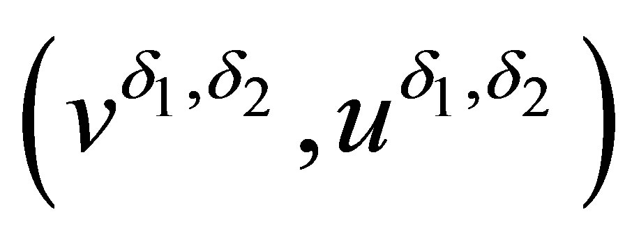 is a weak solution of system (2.14) or satisfies (2.14) in the sense of distributions. For fixed
  (or
(or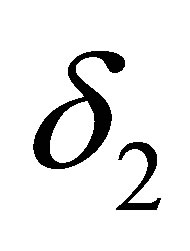 ), and for the generalized functions
 , we may rewrite system (2.14) as
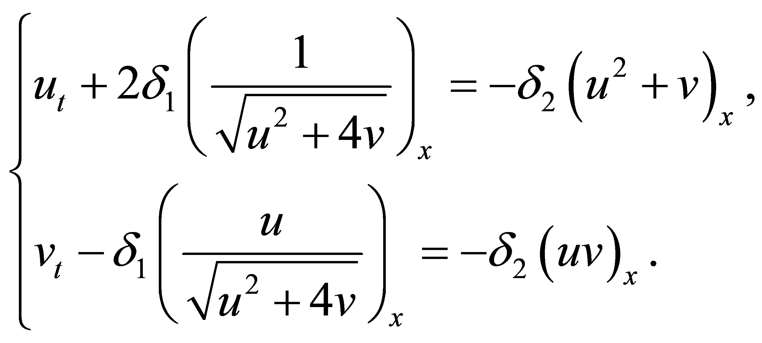 (2.22)
Since the left hand side of (2.22) or system (2.1) is also strictly hyperbolic and genuinely nonlinear, and the functions  are uniformly bounded, independent of
 , so the DiPerna’s result [18] reduces the following convergence
 (2.23)
where the limit 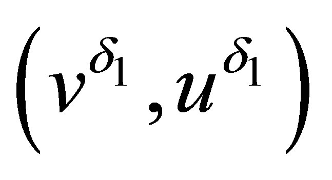 is a weak solution of system (2.1) or satisfies (2.1) in the sense of distributions, which ends the proof of Theorem 1.
3. Acknowledgements
This work was partially supported by the Natural Science Foundation of Zhejiang Province of China (Grant No. LY12A01030 and Grant No. LZ13A010002) and the National Natural Science Foundation of China (Grant No. 11271105).
REFERENCES
- T. Tartar, “Compensated Compactness and Applications to Partial Differential Equations,” In: R. J. Knops, Ed., Research Notes in Mathematics, Nonlinear Analysis and Mechanics, Heriot-Watt Symposium, Vol. 4, Pitman Press, London, 1979.
- F. Murat, “Compacité par Compensation,” Annali della Scuola Normale Superiore di Pisa, Vol. 5, No. 3, 1978, pp. 489-507.
- S. Bianchini and A. Bressan, “Vanishing Viscosity Solutions of Nonlinear Hyperbolic Systems,” Annals of Mathematics, Vol. 161, No. 1, 2005, pp. 223-342. http://dx.doi.org/10.4007/annals.2005.161.223
- J. Glimm, “Solutions in the Large for Nonlinear Hyperbolic Systems of Equations,” Communications on Pure and Applied Mathematics, Vol. 18, No. 4, 1965, pp. 95- 105. http://dx.doi.org/10.1002/cpa.3160180408
- H. Holden and N. H. Risebro, “Front Tracking for Hyperbolic Conservation Laws,” Springer-Verlag, New York, 2002. http://dx.doi.org/10.1007/978-3-642-56139-9
- C. M. Dafermos, “Polygonal Approximations of Solutions of the Initial Value Problem for a Conservation Law,” Journal of Mathematical Analysis and Applications, Vol. 38, No. 1, 1972, pp. 33-41. http://dx.doi.org/10.1016/0022-247X(72)90114-X
- L. Leibovich, “Solutions of the Riemann Problems for Hyperbolic Systems of Quasilinear Equations without Convexity Conditions,” Journal of Mathematical Analysis and Applications, Vol. 45, No. 1, 1974, pp. 81-90. http://dx.doi.org/10.1016/0022-247X(74)90122-X
- C. M. Dafermos, “Hyperbolic Conservation Laws in Continuum Physics,” Grundlehren der Mathematischen Wissenschaften, Vol. 325, Springer Verlag, Berlin, 2001.
- B. L. Keyfitz, “Some Elementary Connections among Nonstrictly Hyperbolic Conservation Laws,” In: Contemporary Mathematics, American Mathematical Society, Providence, 1987, pp. 67-77. http://dx.doi.org/10.1090/conm/060/873532
- Y.-G. Lu, “Convergence of the Viscosity Method for a Nonstrictly Hyperbolic Conservation Laws,” Communications in Mathematical Physics, Vol. 150, No. 1, 1992, pp. 59-64.
- Y.-G. Lu, “Some Results on General System of Isentropic Gas Dynamics,” Differential Equations, Vol. 43, No. 1, 2007, pp. 130-138. http://dx.doi.org/10.1134/S0012266107010132
- Y.-G. Lu, “Global Hölder Continuous Solution of Isentropic Gas Dynamics,” Proceedings of the Royal Society of Edinburgh, Section: A Mathematics, Vol. 123, No. 2, 1993, pp. 231-238. http://dx.doi.org/10.1017/S0308210500025658
- Y.-G. Lu, “Global Existence of Solutions to Resonant System of Isentropic Gas Dynamics,” Nonlinear Analysis, Real World Applications, Vol. 12, No. 5, 2011, pp. 2802- 2810. http://dx.doi.org/10.1016/j.nonrwa.2011.04.005
- Y.-G. Lu, “Existence of Global Bounded Weak Solutions to Non-Symmetric Systems of Keyfitz-Kranzer Type,” Journal of Functional Analysis, Vol. 261, No. 10, 2011, pp. 2797-2815.
- B. Temple, “Systems of Conservation Laws with Invariant Submanifolds,” Transactions of the American Mathematical Society, Vol. 280, No. 2, 1983, pp. 781-795.
- P. D. Lax, “Shock Waves and Entropy,” In: E. Zarantonello, Ed., Contributions to Nonlinear Functional Analysis, Academia Press, New York, 1971, pp. 603-634.
- Y.-G. Lu, “Hyperboilc Conservation Laws and the Compensated Compactness Method,” Chapman and Hall, CRC Press, New York, 2002.
- R. J. DiPerna, “Convergence of Approximate Solutions to Conservation Laws,” Archive for Rational Mechanics and Analysis, Vol. 82, No. 1, 1983, pp. 27-70.
NOTES
*Corresponding author.

