Advances in Pure Mathematics
Vol.3 No.5(2013), Article ID:35060,12 pages DOI:10.4236/apm.2013.35065
The Second Hochschild Cohomology Group for One-Parametric Self-Injective Algebras
Department of Mathematics, Taif University, Taif, KSA
Email: dak12le@hotmail.co.uk
Copyright © 2013 Deena Al-Kadi. This is an open access article distributed under the Creative Commons Attribution License, which permits unrestricted use, distribution, and reproduction in any medium, provided the original work is properly cited.
Received March 12, 2013; revised April 30, 2013; accepted June 23, 2013
Keywords: Hochschild Cohomology; Self-Injective Algebras; Socle Deformation
ABSTRACT
In this paper, we determine the second Hochschild cohomology group for a class of self-injective algebras of tame representation type namely, which are standard one-parametric but not weakly symmetric. These were classified up to derived equivalence by Bocian, Holm and Skowroński in [1]. We connect this to the deformation of these algebras.
1. Introduction
This paper determines the second Hochschild cohomology group for all standard one-parametric but not weakly symmetric self-injective algebras of tame representation type. Bocian, Holm and Skowroński give, in [1], a classification of these algebras by quiver and relations up to derived equivalence. The algebras in [1] are divided into two types, namely the algebra  where
where  are integers such that p,


 and
and 
 and the algebra
  where
where . Thus the second Hochschild cohomology group will be known for all the classes of the algebras given in [1]. We remark that an algebra of the type
  is never isomorphic to an algebra of the type
  as their stable Auslander-Reiten quivers are not isomorphic. We refer the reader to [1] which gives precise conditions for two algebras of the same type
  or
or  to be isomorphic.
We start, in Section 2, by introducing the algebras , for both types, by quiver and relations. Section 3 of this paper describes the projective resolution of [2] which we use to find
 . In the third section, we determine
  for the algebra
 , considering separately the cases
  and
and . The main result in this section is Theorem 4.9, which shows that
  has dimension 1 for
 . This group measures the infinitesimal deformations of the algebra
 ; that is, if
  then
then  has no non-trivial deformations, which is not the case here. We include, in Section 4, Theorem 4.10 where we find a non-trivial deformation
  of
of  associated to our nonzero element
  in
in . This illustrates the connection between the second Hochschild cohomology group and deformation theory. In the final section, we determine
  for
for . The main result in Section 5 is Theorem 5.4 which shows that
 . The results we found in this paper are in contrast to the majority of self-injective algebras of finite representation type (see [3]). Since Hochschild cohomology is invariant under derived equivalence, the second Hochschild cohomology group is now known for the standard one-parametric but not weakly symmetric self-injective algebras of tame representation type which are derived equivalent to the algebra of the type
  or
or .
.
2. The One-Parametric Self-Injective Algebras
In this chapter we describe the algebras of [1]. We start with the algebra . Let K be an algebraically closed field and let
  be integers such that p,

 and
and . From [1, Section 5],
  has quiver
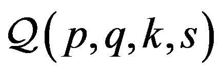 :
:
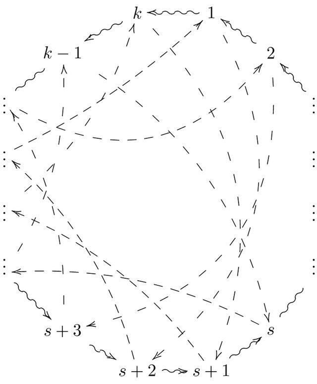
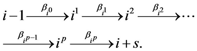
where, for any ,
, 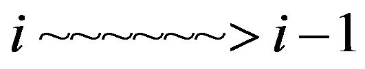 denotes the path
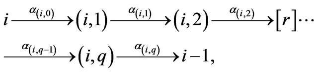
and 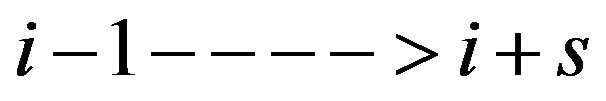 denotes the path
Then 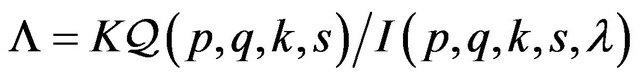 where
where  is the ideal generated by the relations
• ![]() , for
, for •
•  , for
, for •
•  for
for ,
,  ,
,
![]()
![]() for
for ,
,  ,
,
![]()
![]() for
for , and
, and
 where
where .
.
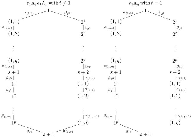
Next we describe the algebra  For
For ,
,  is given in [1, Section 6] by the quiver
 :
:
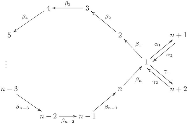
Then 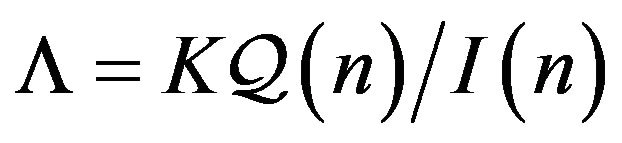 where
where  is the ideal generated by the relations:
1) 
2) 
3) for all 
Note that we write our paths from left to right.
In order to compute , the next section gives the necessary background required to find the first terms of the projective resolution of
  as a
as a  -bimodule. Section 4 and Section 5 uses this part of a minimal projective bimodule resolution for our algebras to determine the second Hochschild cohomology group and provides the main results of this paper.
3. Projective Resolutions
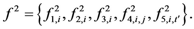
To find the second Hochschild cohomology group , we could use the bar resolution given in [4]. This bar resolution is not a minimal projective resolution of
  as
as  -bimodule. In practice, it is easier to compute the Hochschild cohomology group if we use a minimal projective resolution. So here we use the projective resolution of [2]. More generally, let
  be a finite dimensional algebra, where K is an algebraically closed field,
  is a quiver, and I is an admissible ideal of
 . Fix a minimal set
  of generators for the ideal I. Let
 . Then
 , that is, x is a linear combination of paths
  for
for  and
and  and there are unique vertices v and w such that each path
  starts at v and ends at w for all j. We write
  and
and  Similarly
  is the origin of the arrow a and
  is the end of a.
In [2, Theorem 2.9], it is shown that there is a minimal projective resolution of  as a
as a  -bimodule which begins:
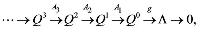
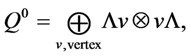
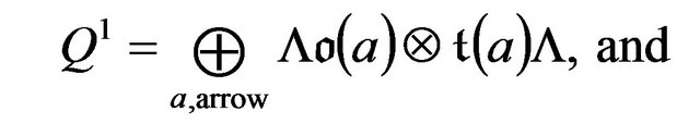
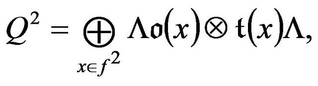
where the projective  -bimodules
  are given by
and the maps ,
,  and
and  are
are  -bimodule homomorphisms, defined as follows. The map
  is the multiplication map so is given by
 . The map
 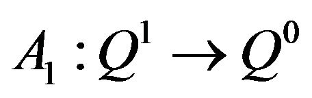 is given by

for each arrow![]() . With the notation for
. With the notation for  given above, the map
 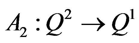 is given by
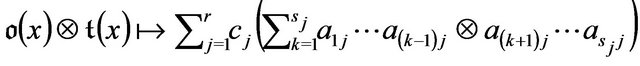 where
where .
.
In order to describe the projective bimodule  and the map
  in the
  -bimodule resolution of
  in [2], we need to introduce some notation from [5]. Recall that an element
  is uniform if there are vertices
  such that
  We write
  and
and . In [5], Green, Solberg and Zacharia show that there are sets
  in
in , for
, for , consisting of uniform elements
  such that
for unique elements  such that
 . These sets have special properties related to a minimal projective
  -resolution of
 , where
  is the Jacobson radical of
 . Specifically the n-th projective in the minimal projective
  -resolution of
  is
is
In particular, to determine the set , we follow explicitly the construction given in [5, §1]. Let
  denote the set of arrows of
 . Consider the intersection
 . Set this intersection equal to some
 . We then discard all elements of the form
  that are in
 ; the remaining ones form precisely the set
 .
.
Thus, for  we have that
 . So we may write
 with
with , such that
  are in the ideal generated by the arrows of
 , and
, and  unique. Then [2] gives that
 and, for
  in the notation above, the component of
  in the summand
  of
of  is
is
Applying  to this part of a minimal projective bimodule resolution of
  gives us the complex
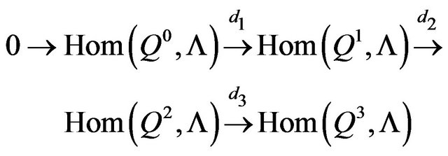
where  is the map induced from
  for
for . Then
Throughout, all tensor products are tensor products over , and we write
  for
for . When considering an element of the projective
  -bimodule
 it is important to keep track of the individual summands of
 . So to avoid confusion we usually denote an element in the summand
  by
by  using the subscript “a” to remind us in which summand this element lies. Similarly, an element
  lies in the summand
 of
of  and an element
  lies in the summand
  of
of . We keep this notation for the rest of the paper.
4.  for
for ![]()
We have given  by quiver and relations in Section 2. However, these relations are not minimal. So next we will find a minimal set of relations
  for this algebra.
Let
![]()
The remaining relations given in Section 2 are all linear combinations of the above relations. For example, the relation ![]() can be written as
can be written as
So this relation is in I and is not in .
.
Proposition 4.1 For  and with the above notation, the minimal set of relations is
In contrast to the majority of self-injective algebras of finite representation type, we will show that the algebra  has non-zero second Hochschild cohomology group (see [3, Theorem 6.5]). Recall that
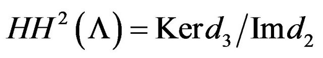 , where
is induced by .
.
First we will find . Since
 let
let  so that
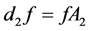 . We consider the cases
  and
and  separately.
Let  and
and

where all coefficients  for
for 
 for
for 
 Now we find
 .
.
First we have,
Similarly for ,
,
For the remaining terms, 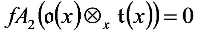 where
where 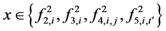 for all
 ,
,
 and
and .
.
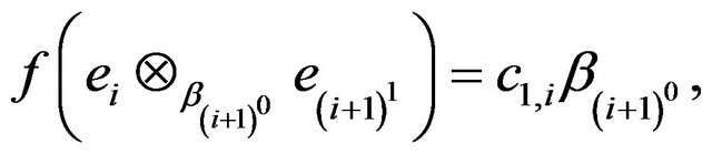
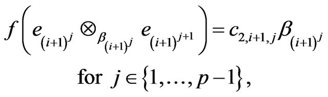
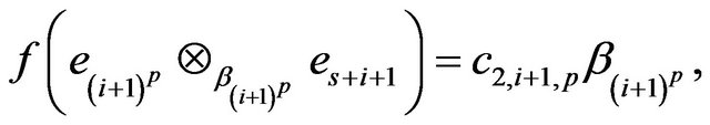
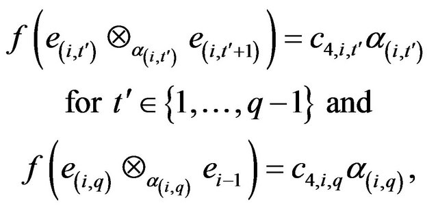
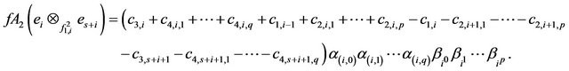
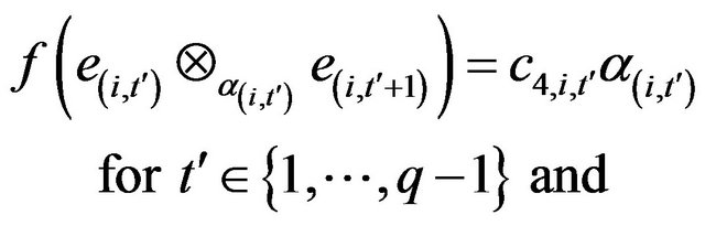
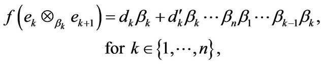
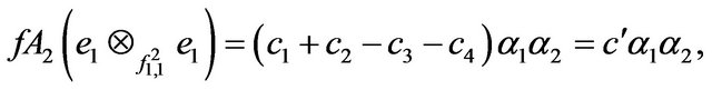
Let
for  and
and
for 
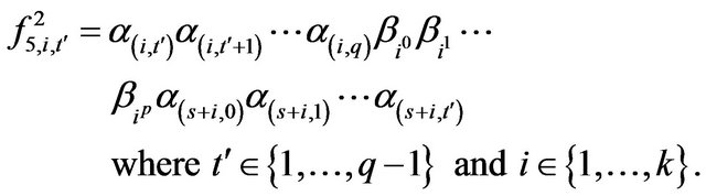
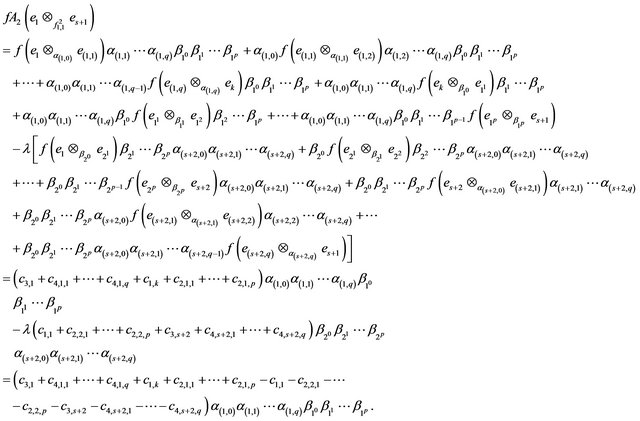
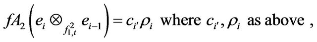
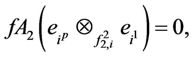
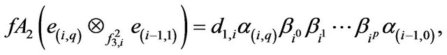
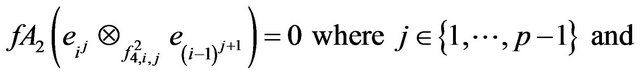
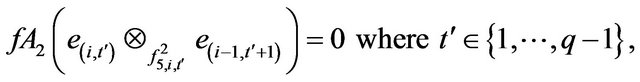
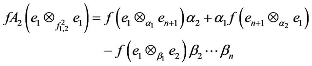
Thus for  and
and , fA2 is given by
where  with
with . So
. So
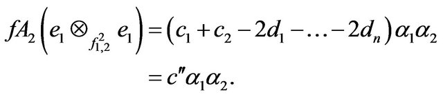
For , we let


where for all  the coefficients
  for
for 
 for
for 
 are in
Then we can find  for
for  in the same way as the previous case to see that it is given by
where  with
with . Note that there is no dependency between the
  So
So 
Proposition 4.2 If , we have
 If
If , we have
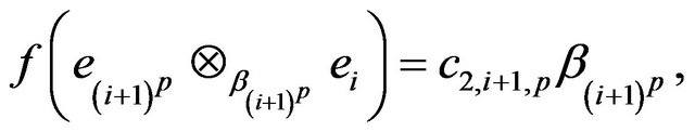
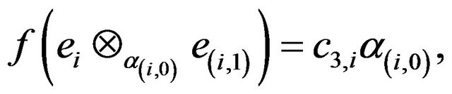
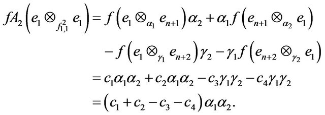
Next we find  and again consider the two cases separately. Let
  and
and  . Then
  is defined by
where .
.
Therefore  Hence,
For  and
and ,
,  is given by
where  are in K for
  Thus
Thus 
Proposition 4.3 If , we have
 If
If ,
,

Corollary 4.4 If , we have
 . If
. If ,
, 
In order to find Kerd3 and hence determine  we start by giving a non-zero element in
  for all s.
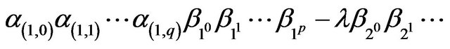
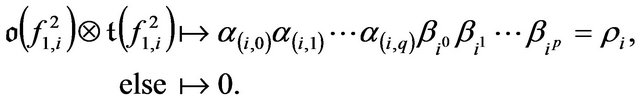
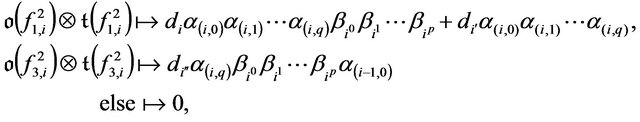
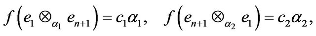
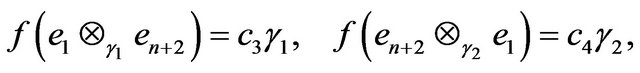
Proposition 4.5 Define  by
by
Then ![]() is in
is in .
.
Proof. We note that  so
so ![]() is a non-zero map. To show that
is a non-zero map. To show that  we show that
 . First, observe that
 ![]() and
and  Hence
Hence . Similarly we have
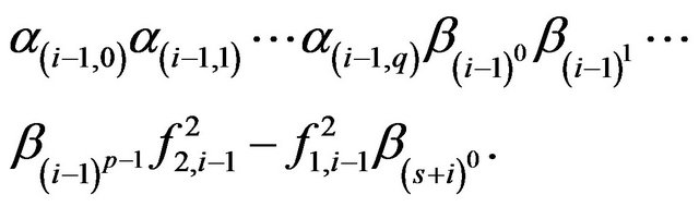
Recall that ![]() where
where
 and
and  are in the ideal generated by the arrows. For
  the component of
 in
in  is
is
Then
Thus
As  is in the arrow ideal of
 ,
,  So we have
  Similarly
 as
as  Therefore
 for all
  so
so . Thus
  as required.
Theorem 4.6 For  where
where  are positive integers,
  ,
,  with
with
 and
and , we have
 .
.
Proof. Consider the element  of
of 
where ![]() is given as in Proposition 4.5 by
is given as in Proposition 4.5 by
Suppose for contradiction that  Then
Then . So
. So  and so
 . Also
  where
where  Then
Then  where
where  But this contradicts having
 . Therefore
 , that is,
 . So
. So  is a nonzero element in
 □
□
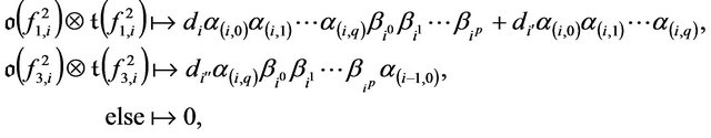
Note that we can also define maps  by
by
for . However,
  all represent the same element
  of
of .
.
As we have found a non-zero element in  we know that
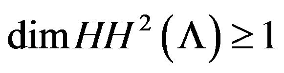 . In the case
 we have the following result, the proof of which is immediate from Proposition 4.2, Corollary 4.4 and Theorem 4.6.
Proposition 4.7 For  where
where , we have
  and
and

For the case , we need more details to find
 . Following [5] we may choose the set
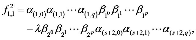
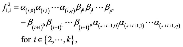
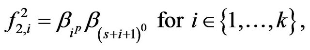
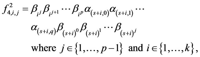
  to consist of the following elements:
 where
where

![]()

![]()
![]()

![]()

![]()


![]()


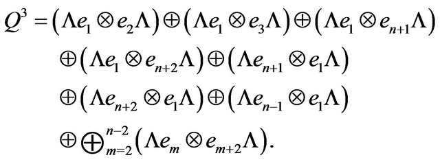
Thus the projective bimodule  is
is 
Now we determine  in the case
 . Let
. Let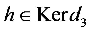 , so
, so  and
and . Recall that for
 ,
,  is given by
where  are in
 .
.
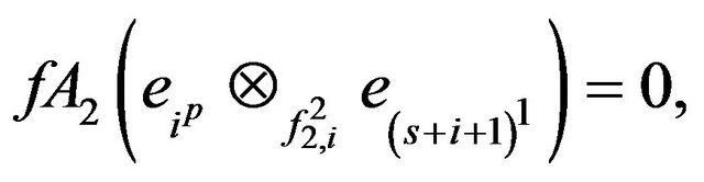
Then for , we have
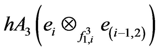
In a similar way we can show that .
.
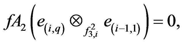
For , we have

As  we have
  for
for .
.
Similarly it can be shown that
so that .
.
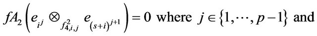
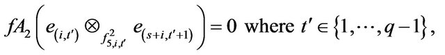
We also have 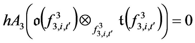 for
for
 and
and 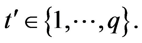 Finally, putting
does not give any new information for ,
, .
.
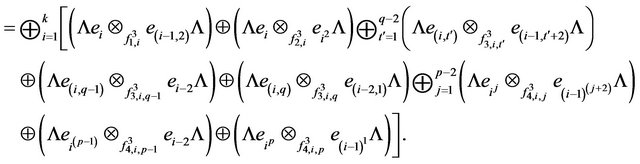
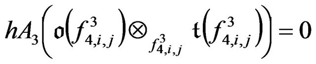
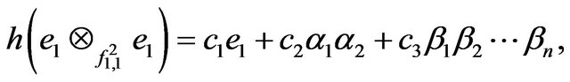
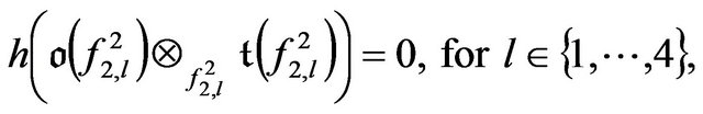
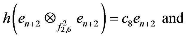
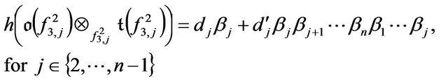
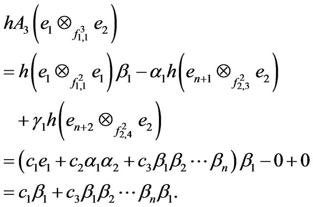
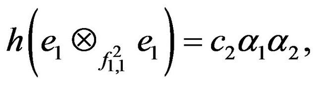
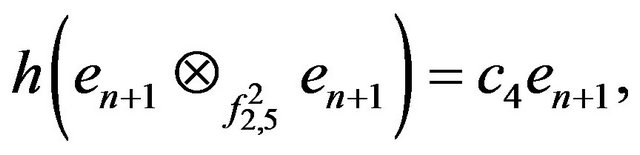
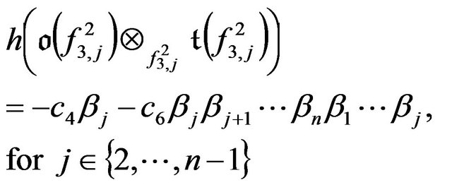
Thus h is given by
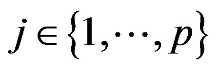
where  for
for  are in K. It is clear that there is no dependency between
 , and therefore
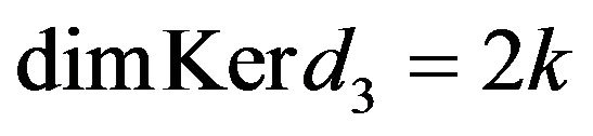 .
.
Proposition 4.8 For  and
and , we have
Using Propositions 4.2, 4.7, 4.8 and Theorem 4.6 we get the main result of this section.
Theorem 4.9 For  where p, q, s, k are integers such that p,

 and
and , we have
We conclude this section by giving a deformation of  which arises from the non-zero element
  in
in .
.
Let . Recall that
 . We introduce a new parameter
  and define the algebra
  to be the algebra
  where
where  is the ideal generated by the following elements:
1)  where
where 
2) for all ,
,  where
where 
3)  for all arrows a with
 4)
4)  for all arrows a with
We now need to show that  to verify that
  is indeed a deformation of
 . First of all, it is clear that
  for all t and for all vertices ei with
 . Now we consider
  and
and  with
with![]() , and
, and  with
with![]() . These projective modules are described as follows:
. These projective modules are described as follows:
In each case we see that
for all t. Hence . Moreover, when
 ![]() the algebras
the algebras  and
and  are not isomorphic since, in this case,
  is not self-injective. Thus we have found a non-trivial deformation of
 .
.
Theorem 4.10 With  and
and  as defined above, then
  is a non-trivial deformation of
 . Moreover, the algebras
  and
and  are socle equivalent.
5.  for
for 
We have given the algebra  by quiver and relations in Section 2. Note that these relations are not minimal. So we will find a minimal set of relations
  for this algebra.
Let
The remaining relation  can be written as
 . So this relation is in I and is not in
 .
.
Proposition 5.1 For  and with the above notation, the minimal set of relations is
Recall that the projective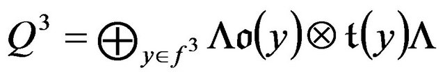 . Thus we have
(We note that the projective  is also described in [4] although Happel gives no description of the maps in the
  -projective resolution of
 .) Following [2], and with the notation introduced in Section 3, we may choose the set
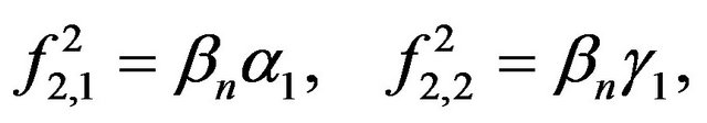
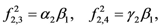
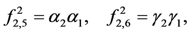
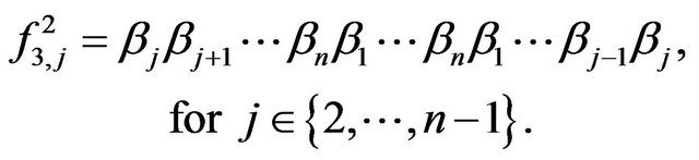
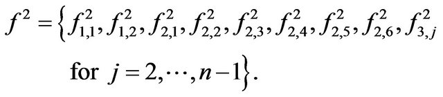
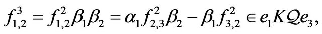
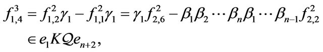
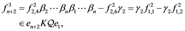
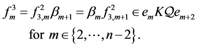
  to consist of the following elements:
with  where
where


We know that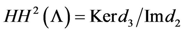 . First we will find
 . Let
. Let  and so write
where 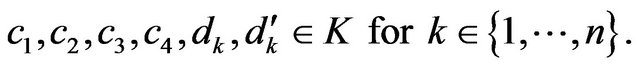
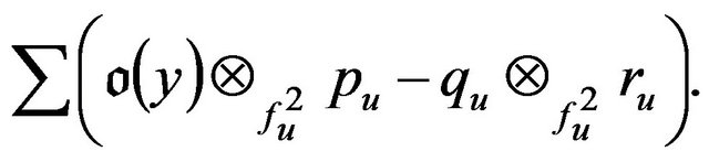
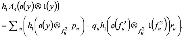
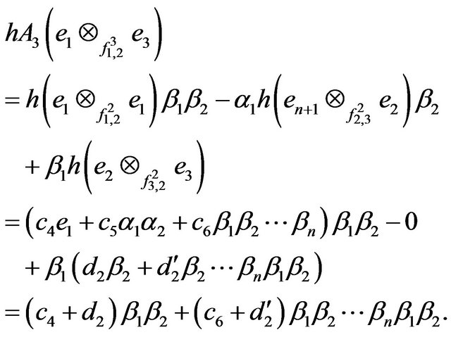
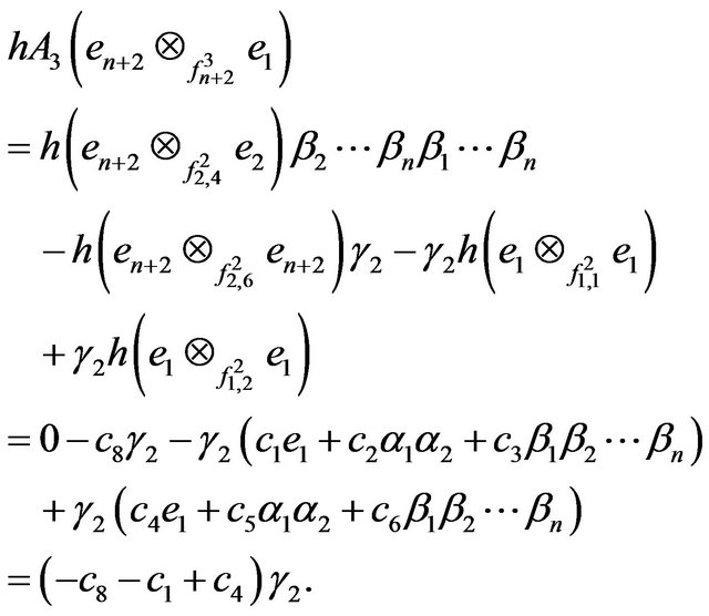
Now we find . We have
Also
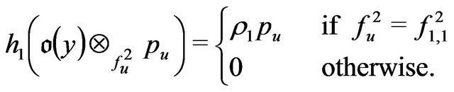
We can show by direct calculation that
 for all
 .
.
Thus  is given by
So .
.
Proposition 5.2 For , we have
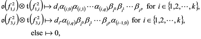
Now we determine . Let
. Let , so
, so 
 and
and . Then
  is given by


for some  for
for 
Then
As  we have
  and
and 
As  we have
  and
and . So
. So  and
and 
Next,
So we have  and hence
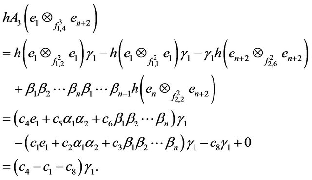
Therefore  as
as 
Thus again we have 
As  above, we have
 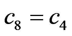 as we already know.
Also
So we have 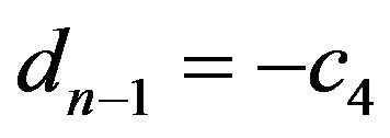 and
and 
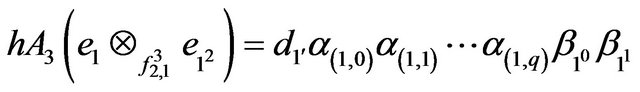
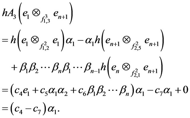
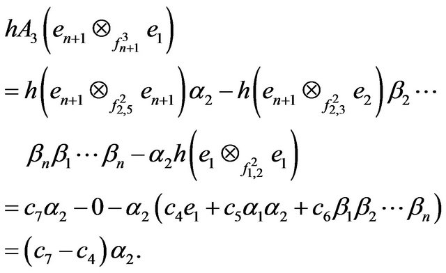
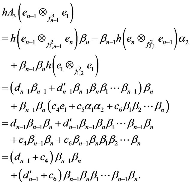
Finally, for , we have
Therefore we have  and
and . Hence
  and
and  for
for  as we have above
 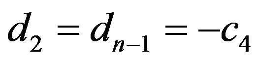 and
and 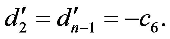
Thus  is given by


for some 
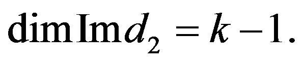
Proposition 5.3 For , we have
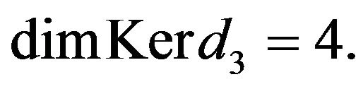
Therefore

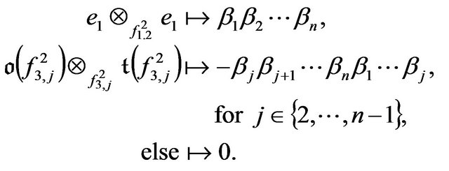
and a basis is given by the maps  and
and  where
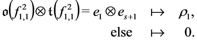
where  is given by
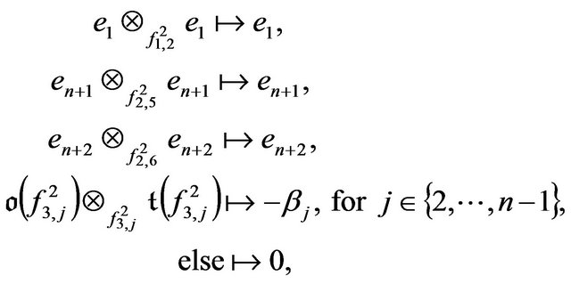
 is given by
From Proposition 5.2 and Proposition 5.3 we get the main result of this section.
Theorem 5.4 For  with
with  we have
To connect this with deformations we use a similar discussion as Section 4. We introduce the parameter  and define the algebra
  to be the algebra
  where
where  is the ideal generated by the following elements:
1) 
2) 
3) 
4) 
We can show that . Hence this algebra has no non-trivial deformation.
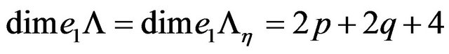
From Theorem 4.9 and Theorem 5.4 we have now found  for all standard one-parametric but not weakly symmetric self-injective algebras of tame representation type.
6. Acknowledgements
I thank Prof. Nicole Snashall for her encouragement and helpful comments.
REFERENCES
- R. Bocian, T. Holm and A. Skowroński, “Derived Equivalence Classification of One-Parametric Self-Injective Algebras,” Journal of Pure and Applied Algebra, Vol. 207, No. 3, 2006, pp. 491-536. doi:10.1016/j.jpaa.2005.10.015
- E. L. Green and N. Snashall, “Projective Bimodule Resolutions of an Algebra and Vanishing of the Second Hochschild Cohomology Group,” Forum Mathematicum, Vol. 16, No. 1, 2004, pp. 17-36. doi:10.1515/form.2004.003
- D. Al-Kadi, “Self-Injective Algebras and the Second Hochschild Cohomology Group,” Journal of Algebra, Vol. 321, No. 4, 2009, pp. 1049-1078. doi:10.1016/j.jalgebra.2008.11.019
- D. Happel, “Hochschild Cohomology of Finite-Dimensional Algebras,” Lecture Notes in Mathematics, SpringVerlag, Berlin, 1989. doi:10.1090/S0002-9947-01-02687-3
- E. L. Green, Ø. Solberg and D. Zacharia, “Minimal Projective Resolutions,” Transactions of the American Mathematical Society, Vol. 353, No. 7, 2001, pp. 2915-2939. doi:10.1007/BFb0084073