ABSTRACT

This paper studies the global behavior to 3D focusing nonlinear Schrödinger equation (NLS), the scaling index here is, which is the mass-supercritical and energy-subcritical, and we prove under some condition the solution is globally well-posed and scattered. We also show that the solution “blows-up in finite time” if the solution is not globally defined, as we can provide a depiction of the behavior of the solution, where T is the “blow-up time”.

1. Introduction

Consider the Cauchy problem for the nonlinear Schrö- dinger equation (NLS) in dimensions d = 3:

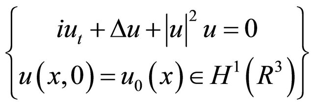(1.1)

where is a complex-valued function in . The initial-value problem is locally well-posed in.

In this paper we will study the focusing (NLS) problem, which is the mass-supercritical and energy-subcritical, where

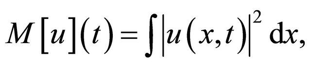
The Equation (1.1) has mass where

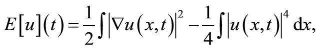
Energy where

and Momentum where

.

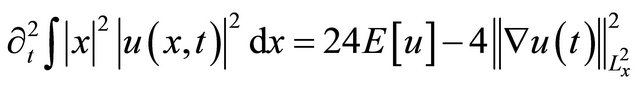
If, then u satisfies

(1.2)

Equation (1.2) is said to be the Virial identity.

The Equation (1.1) has the scaling:

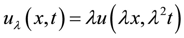
and also this scaling is a solution if is a solution.

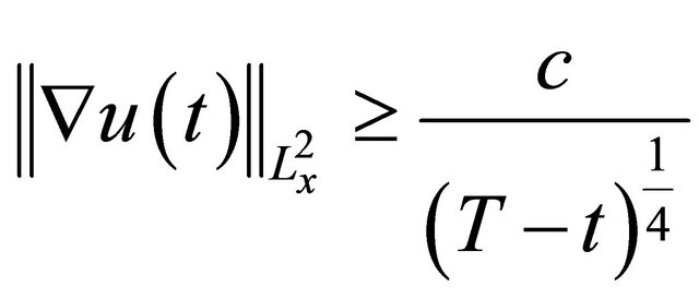
Moreover, u₀ is a solution that is globally defined by u, if it is globally defined, and it does scatter (See [1,2]). We say the solution “blows-up in finite time”. If the solution is not globally defined, as, we can provide a depiction of the behavior of the solution, where T is the “blow-up time”. It follows from the H¹ local theory optimized by scaling, that if blow-up in finite-time T > 0 happens, (see [3] or [4]), then there is a lower-bound on the “blow-up rate”:

(1.3)

for some constant c. Thus, to prove global presence, it suffices to prove a global axiomatic bound on.

From the Strichartz estimates, there is a constant such that if , then the solution is globally defined and scattered.

Note that the quantities and

are also scale-invariant (See also [5]).

Let then u solves (1.1) as long as

solves the nonlinear elliptic equation

(1.4)

Equation (1.4) has an infinite number of solutions in. The solution of minimal mass is denoted by and for the properties of see [3,5,6].

Under the condition, solutions to (1.1) globally exist if u₀ satisfies;

(1.5)

and there exist such that

.

Theorem 1.1. Let, and let be the corresponding solution to (1.1) in H¹. Suppose

(1.6)

If then u scatters in H¹.

The argument of [6] in the radial case followed a strategy introduced by [7] for proving global well-posedness and scattering for the focusing energy-critical NLS. The beginning used a contradiction to the argument: suppose the sill for scattering is strictly below that claimed. This uniform localization enabled the use of a local Virial identity to be established, with the support of the sharp Gagliardo-Nirenberg inequality, an accurately positive lower bound on the convexity (in time) of the local mass of u_c Mass conservation is then violated at enough large time.

We show in this paper, that the above program carries over to the non-radial setting with the extension of two key components.

Theorem 1.2. Suppose the radial H¹ solution u to (1.1) blows-up at time Then either there is a non-absolute constant such that, as

(1.7)

or there exists a sequence of times such that for an absolute constant

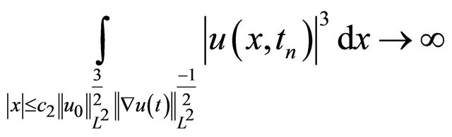(1.8)

From (1.3), we have that the concentration in (1.7) satisfies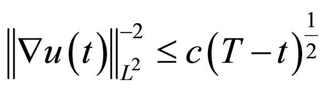, and the concentration in (1.8) satisfies 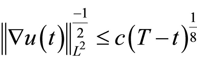(For more additional information see [8-10]).

Notation

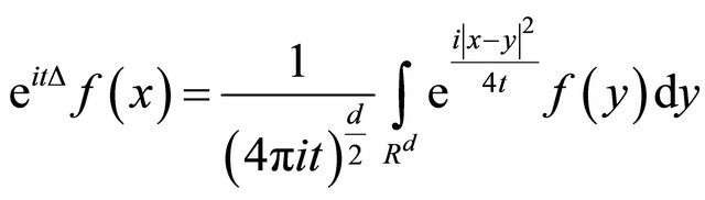
Let be the free Schrödinger propagator, and let, with be linear equation, a solution in physical space, is given by:

and in frequency space

In particular, they save the Farewell homogeneous Sobolev norms and obey the dispersive inequality

(1.9)

For all times.

Let be a radial function, so that, for and for, Define the inner and outer spatial localizations of at radius as

Let be a radial function so that,

for and for then

, and define the inner and outer indecision localizations at radius of u₁ as

and

(the and radii are chosen to be consistent with the assumption, since. In reality, this is for suitability only; the argument is easily proper to the case where is any number). We note that the indecision localization of is inaccurate, though decisively we have;

(1.10)

2. Proof of Theorem 1.2

In this section we discuss a proof of Theorem (1.2).

Proposition 2.1. Let u be an H¹ radial solution to (1.1) that blows-up in finite. Let

and, (Where c₁ and c₂ are absolute constants), and as characterized in the paragraph above.

1) There exists an absolute constant such that

(2.1)

2) Let us assume that there exists a constant such that. Then

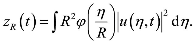
(2.2)

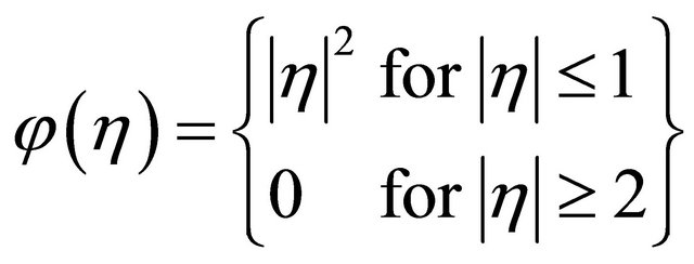
for some absolute constant c > 0, where is a stance function such that

We recall, an “exterior” estimate, usable to radially symmetric functions only, originally due to [11]:

(2.3)

where c is independent of R > 0. We recall the generally usable symmetric functions and for any function

(2.4)

(2.3), (2.4) are Gagliardo-Nirenberg estimates for functions on.

Proof of Prop 2.1: Since by (1.3), as by energy conservation, we have

Thus, for t to be large enough to close to T

(2.5)

By (2.3), the selection of and mass conservation;

(2.6)

where c₁ in the definition of has been selected to obtain the factor here. By Sobolev embedding, (1.10), and the selected

(2.7)

where c₂ in the definition of has been selected to obtain the factor here. Bring together (2.5), (2.6), and (2.7), to obtain

(2.8)

By (2.8) and (2.4), we obtain (2.1), completing the proof of part (1) of the proposition.

To prove part (2), we assume by (2.8)

There exists for which at least of this supremum is attained. Thus,

where we used Hölder’s inequality in the last step. By the selected, we obtain (2.2). To complete the proof, it keeps to obtain the remind control on which will be a consequence of the radial supposition and the supposed bound

Assume along a sequence of times Assume the spherical annulus;

And inside A place disjoint balls, at radius both the radius, centered on the sphere. By the radiality supposition, on all ball B, we have

, and hence on the annulus A,

.

which contradicts the assumption.

We now point out how to obtain Theorem 1.2 as a consequence.

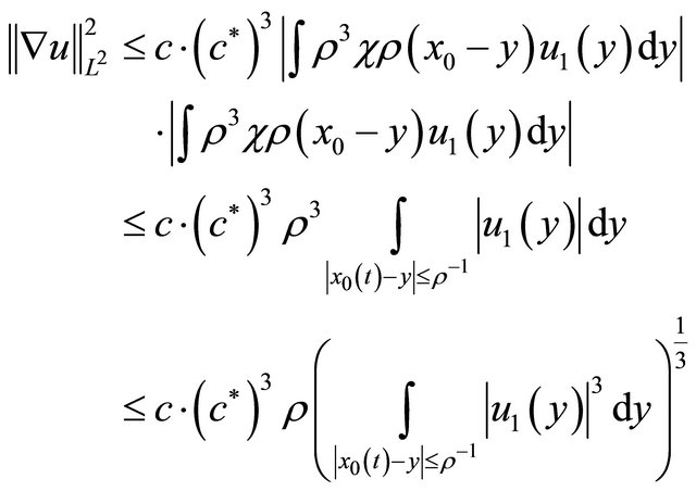
Proof of Theorem 1.2. By part (1) of Prop. 2.1 and the standard convolution inequality:

.

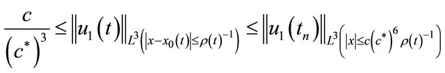
If is not bounded, then there exists a sequence of times such that Since

, we have (1.8) in Theorem 1.2;

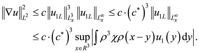
on the other hand, if, for some c^*, as t ® Twe have (2.2) of Prop. 2.1. Since, we have

which gives (1.7) in Theorem 1.2.

3. Strichartz Estimates

In this section we show local theory and Strichartz estimates.

Strichartz Type Estimates

We say the pair is Strichartz admissible if

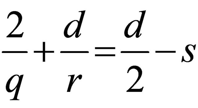, with, and. And the pair is -passable if, , or.

As habitual we denote by the Hölder conjugates of q and r consecutive (i.e.).

Let

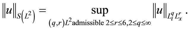
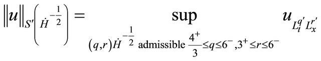
We consider dual Strichartz norms. Let

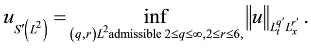
where is the Hölder dual to. Also define

The Strichartz estimates are:

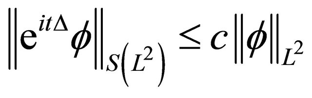
and

.

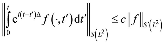By bring together Sobolev embedding with the Strichartz estimates, we obtain

and

(3.1)

We must also need the Kato inhomogeneous Strichartz estimate [12].

. (3.2)

To point out a restriction to a time subinterval , we will write or.

Proposition 3.1 Assume. There is such that if, then u solving (1.1) is global (in) and

,

.

(Observe that, by the Strichartz estimates, the assumptions are satisfied if).

Proof. Define

.

Applying the Strichartz estimates, we obtained

and

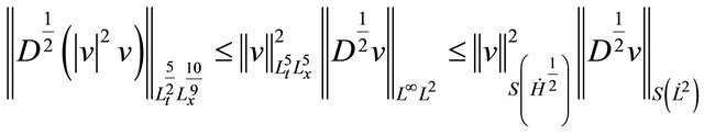
We apply the Hölder inequalities and fractional Leibnitz [13] to get

Let

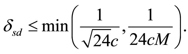
Then where

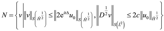
and is a contraction on N.

Proposition 3.2. If is global with globally finite Strichartz norm 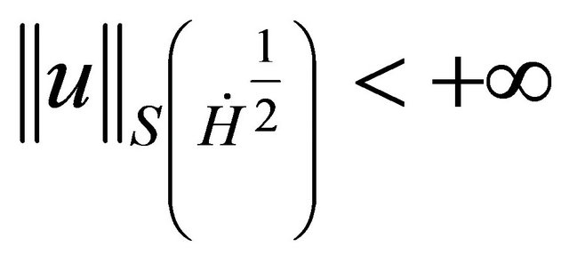and a uniformly bounded H¹ norm then scatters in H¹ as.

Meaning that there exist such that

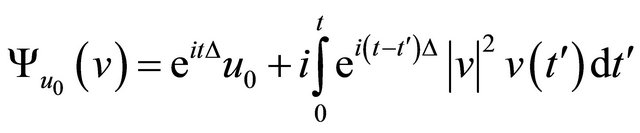
Proof. Since resolves the integral equation

we have

(3.3)

where

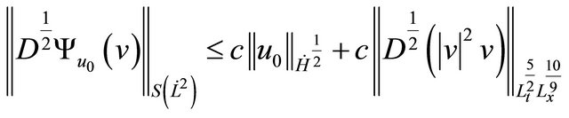
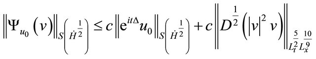
Apply the Strichartz estimates to (3.3), to get

As above inequality get the claim.

4. Some Lemma

4.1. Here We Discuss the Precompactness of the Flow Implies Regular Localization

Let u be a solution to (1.1) such that

(4.1)

is precompact in H¹. Then for each there exist  R > 0 so that for all

We proof (4.2) by contradiction, there exists and a sequence of times and by changing the variables,

(4.3)

Since K is precompact, there exists, such that in H¹, by (4.3),

Which is a contradiction with the fact that The proof is complete.

Lemma 4.1. Let u be a solution of (1.1) defined on, such that and K such as in (4.1) is precompact in H¹, for some continuous function then;

(4.4)

Proof. Suppose that (4.4) does not hold. Then there exists a sequence, such that for some ε₀ > 0. Retaining generality, we assume For R > 0, let

i.e. is the first time when arrives at the boundary of the ball of radius R. By continuity of, the value is well-defined. Furthermore, the following hold:

1)

2)

3).

Let and We note that, which combined with, gives. Since and, we have Thus We can disregard. We will concentrate our work on the time interval, and we will use in the proof:

1) we have

2)

3) and

By the precompactness of K and (4.2) it follows that for any, there exists, such that for any

(4.5)

We will select ε later; for let be such that for, for

, , and for

. Let

Then for and For R > 0, set Let be the truncation center of mass given by

Then, where

Observe that for. By the zero momentum property

.

Thus,

By Cauchy-Schwarz, we obtain;

(4.6)

Set Observe that for and

, we have, and thus

(4.6), (4.5) give

(4.7)

We now obtain an upper bound for and a lower bound for

Hence, by (4.5) we have

(4.8)

For, we divide as

To deduce the expression for I, we observed that

And use (4.5) to obtain

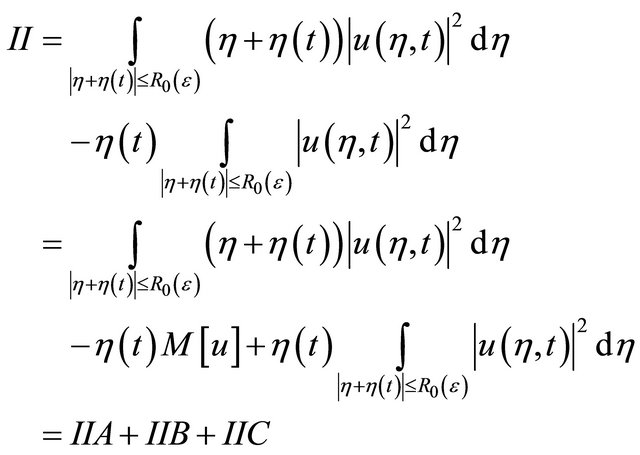
For II we first observe that,

and thus

We rewrite II as

Trivially, and by (4.5)

.

Thus,

Taking, we can get

(4.9)

Combining (4.7), (4.8), and (4.9), we have

Suppose and use to obtain

Since we have

(Assume) take, as since we get a contradiction.

4.2. We Now Prove the Following Rigidity Theorem

Lemma 4.2. If (1.5) and (1.6) hold, then for all t

(4.10)

where. We have also the bound for all t;

(4.11)

The hypothesis here is except if In fact,

Theorem 4.3. Assume satisfies,

(4.12)

and

(4.13)

Let u be the global H¹ solution of (1.1) with initial data u₀ and assume that is precompact in H¹. Then .

Proof. Let be redial with

.

For R > 0, we define

Then

By the Hölder inequality:

(4.14)

By calculation, we have the local Virial identity

Since is radial we have

(4.15)

where

Thus, we obtain

(4.16)

Now discuss for R chosen appropriate large and selection time interval where. By (4.15) and (4.11) we have

(4.17)

Set in (4.2), , such that

(4.18)

Choosing Then (4.16), (4.17) and

(4.18) imply that for all,

(4.19)

By Lemma 4.1, there exists such that for all we have with By taking R =, we obtain that (4.18) holds for all . Integrating (4.19) over we obtain

(4.20)

On the other hand, for all, by (4.10) and (4.14), we have

(4.21)

Combining (4.20) and (4. 21), we obtained

It is important to mention that and are constant depending only on, and.

Putting and setting, we obtain a contradiction except if, which implies

REFERENCES

- T. T. Tao, “On the Asymptotic Behavior of Large Radial Data for a Focusing Non-Linear Schrödinger Equation,” Dynamics of Partial Differential Equations, Vol. 1, No. 1, 2004, pp. 1-48.
- T. Tao, “A (Concentration-)Compact Attractor for High- Dimensional Non-Linear Schrödinger Equation,” Dynamics of Partial Differential Equations, Vol. 4, No. 1, 2007, pp. 1-53.
- T. Cazenave, “Semilinear Schrödinger Equations. Courant Lecture Notes in Mathematics,” New York University, Courant Institute of Mathematical Sciences, New York, American Mathematical Society, Providence, 2003.
- T. Tao, “Nonlinear Dispersive Equations: Local and Global Analysis,” CBMS Regional Conference Series in Mathematics, Published for the Conference Board of the Mathematical Sciences, Washington DC, American Mathematical Society, Providence, 2006.
- M. Weinstein, “Nonlinear Schrödinger Equations and Sharp Interpolation Estimates,” Communications in Mathematical Physics, Vol. 87, No. 4, 1982, pp. 567-576.
- J. Holmer and S. Roudenko, “A Sharp Condition for Scattering of the Radial 3D Cubic Nonlinear Schrödinger Equations,” Communications in Mathematical Physics, Vol. 282, No. 2, 2008, pp. 435-467.
- C. E. Kenig and F. Merle, “Global Well-Posedness, Scattering, and Blow-Up for the Energy-Critical Focusing Nonlinear Schrödinger Equation in the Radial Case,” Inventiones Mathematicae, Vo. 166, No. 3, 2006, pp. 645- 675.
- J. Colliander, M. Keel, G. Staffilani, H. Takaoka and T. Tao, “Global Existence and Scattering for Rough Solutions of a Nonlinear Schrödinger Equation on R3,” Communications on Pure and Applied Mathematics, Vol. 57, No. 8, 2004, pp. 987-1014.
- T. Hmidi and S. Keraani, “Blowup Theory for the Critical Nonlinear Schrödinger Equations Revisited,” International Mathematics Research Notices, Vol. 2005, No. 46, 2005, pp. 2815-2828. doi:10.1155/IMRN.2005.2815
- F. Merle and Y. Tsutsumi, “L2 Concentration of Blow-Up Solutions for the Nonlinear Schrödinger Equation with Critical Power Nonlinearity,” Journal of Differential Equations, Vol. 84, No. 2, 1990, pp. 205-214.
- W. A. Strauss, “Existence of Solitary Waves in Higher Dimensions,” Communications in Mathematical Physics, Vol. 55, No. 2, 1977, pp. 149-162.
- D. Foschi, “Inhomogeneous Strichartz Estimates,” J. Hyper. Diff. Eq., Vol. 2, No. 1, 2005, pp. 1-24.
- C. Kenig, G. Ponce and L. Vega, “Well-Posedness and Scattering Results for the Generalized Korteweg-De Vries Equation via the Contraction Principle,” Communications on Pure and Applied Mathematics, Vol. 46, No. 4, 1993, pp. 527-620.
- S. Keraani, “On the Defect of Compactness for the Strichartz Estimates of the Schrödinger Equation,” Journal of Differential Equations, Vol. 175, No. 2, 2001, pp. 353- 392. doi:10.1006/jdeq.2000.3951
- E. Donley, N. Claussen, S. Cornish, J. Roberts, E. Cornell and C. Wieman, “Dynamics of Collapsing and Exploding Bose-Einstein Condensates,” Nature, Vol. 412, No. 6844, 2001, pp. 295-299. doi:10.1038/35085500
- C. Sulem and P.-L. Sulem, “The Nonlinear Schrödinger Equation. Self-Focusing and Wave Collapse,” Applied Mathematical Sciences, Vol. 139, 1999.
- M. Vilela, “Regularity of Solutions to the Free Schrö- dinger Equation with Radial Initial Data,” Illinois Journal of Mathematics, Vol. 45, No. 2, 2001, pp. 361-370.
- L. Bergé, T. Alexander and Y. Kivshar, “Stability Criterion for Attractive Bose-Einstein Condensates,” Physical Review A, Vol. 62, No. 2, 2000, 6 p.
- P. Bégout, “Necessary Conditions and Sufficient Conditions for Global Existence in the Nonlinear Schrödinger Equation,” Advances in Applied Mathematics and Mechanics, Vol. 12, No. 2, 2002, pp. 817-827.