World Journal of Mechanics
Vol.04 No.02(2014), Article ID:42982,16 pages
10.4236/wjm.2014.42007
Methodology for Comparing Coupling Algorithms for Fluid-Structure Interaction Problems
Jason P. Sheldon*, Scott T. Miller, Jonathan S. Pitt
Applied Research Laboratory, The Pennsylvania State University, State College, USA
Email: *Jason.P.Sheldon@psu.edu, scott.miller@psu.edu, jonathan.pitt@psu.edu
Copyright © 2014 Jason P. Sheldon et al. This is an open access article distributed under the Creative Commons Attribution License, which permits unrestricted use, distribution, and reproduction in any medium, provided the original work is properly cited. In accor- dance of the Creative Commons Attribution License all Copyrights © 2014 are reserved for SCIRP and the owner of the intellectual property Jason P. Sheldon et al. All Copyright © 2014 are guarded by law and by SCIRP as a guardian.
ABSTRACT
The multi-physics simulation of coupled fluid-structure interaction problems, with disjoint fluid and solid do- mains, requires one to choose a method for enforcing the fluid-structure coupling at the interface between solid and fluid. While it is common knowledge that the choice of coupling technique can be very problem dependent, there exists no satisfactory coupling comparison methodology that allows for conclusions to be drawn with respect to the comparison of computational cost and solution accuracy for a given scenario. In this work, we de- velop a computational framework where all aspects of the computation can be held constant, save for the method in which the coupled nature of the fluid-structure equations is enforced. To enable a fair comparison of coupling methods, all simulations presented in this work are implemented within a single numerical framework within the deal.ii [1] finite element library. We have chosen the two-dimensional benchmark test problem of Turek and Hron [2] as an example to examine the relative accuracy of the coupling methods studied; however, the compar- ison technique is equally applicable to more complex problems. We show that for the specific case considered herein the monolithic approach outperforms partitioned and quasi-direct methods; however, this result is prob- lem dependent and we discuss computational and modeling aspects which may affect other comparison studies.
Keywords
Fluid-Structure Interaction; FSI; Finite Element Method; Monolithic Coupling; Partitioned Coupling; Dirichlet-Neumann Coupling; Multi-Physics
1. Introduction
*Corresponding author.
1Mesh motion [3] is another challenging research area for ALE-based methods. For this work, we assume that a mesh motion strategy is chosen and fixed for our coupling types, and as such studies of optimal mesh motion strategies are outside of the current scope.
In this work, we focus on constructing a numerical framework in which algorithms for solving the class of engineering problems commonly referred to as Fluid- Structure Interaction (FSI) problems can be benchmarked and compared in a consistent and quantitative manner. The primary challenge in finding a numerical solution to a FSI problem is not in solving the field equations over either the solid of fluid components of the domain, but rather handling the compatibility conditions that must be enforced on the interface between these components.1 Recently, two primary strategies for enforcing this coupl- ing in the Arbitrary Lagrangian-Eulerian (ALE) frame- work have emerged: solving the solid and fluid compo- nents of the domain separately, while iteratively passing information between them, and a simultaneous solution of all field equations at once. The former method is referred to in this work as “partitioned”, and the latter as “monolithic”.
The choice of coupling strategy is an important deci- sion to make from the start of any endeavor to implement a numerical ALE framework for the simulation of fluid- structure interaction, as it places inherent constraints on the entire effort moving forward. On one hand, an author must be sure to choose an approach that allows for all of the relevant physics to be captured, but must also con- sider the performance of the resulting computer code, the ease of implementation, and its ability to address prob- lems of interest. If one turns to the work of other authors for guidance, conflicting statements can be found re- garding the performance of various coupling approaches. In addition to this, there is seemingly conventional wis- dom in the community today that partitioned approaches are faster than their monolithic counterparts due to the optimized nature of the individual component solvers and smaller systems inverted by the linear solvers [4-7]; however, these notions have been challenged in [8]. There is agreement within the FSI community that, in general, the choice of coupling type is problem depen- dent, although no specific guidance exists on exactly when a coupling strategy should be preferred.
Michler et al. [9] state that in a simple one dimensional FSI problem “the computational cost of the monolithic procedure is three to four times the one of the partitioned procedure;” however, he does not hold each approach to the same convergence tolerance. In fact, he requires more strict convergence of the monolithic solver, which con- tributes to its longer run time. In contrast, he later hypo- thesizes that for more complex problems the monolithic approach would be superior in a comparison of computa- tional cost for a desired accuracy against his partitioned method.
Degroote et al. [6] utilize ADINA [10], a commercial finite element software package, to compare partitioned and monolithic FSI. They claim that ADINA converges both methods to the same tolerances, for the norms of displacement and force on the interface; however, it is unclear exactly what convergence criterion is used as no equations or methods are presented. They find that for certain cases their partitioned method requires half the computational time of their monolithic method, while for other cases it requires as much as four times the compu- tational time of the monolithic method, and in some cas- es, the partitioned method does not converge at all.
On the other hand, Heil et al. [8] use the open source finite element library OOMPH-LIB [11] to compare par- titioned and monolithic methods. In their tests, they found that, in terms of computation time required, mono- lithic methods outperform partitioned methods when FSI effects were significant and that this behavior was ampli- fied with proper pre-conditioners. Again, it is unclear exactly what parameters they use to signify convergence. They claim that the convergence criterion is either the maximum global residual, or the maximum change in position of nodes between iterations; however, in all of their cases they do not require the partitioned method to converge to the same tolerances as the monolithic me- thod.
As can be seen by these examples, although there has been past work in comparing coupling techniques, there is no clear agreement on which method is optimal for a given problem. To aid in providing clarity to this situa- tion, we have developed an ALE-based framework that can hold constant many of the confounding factors and can focus solely on the fluid-structure coupling metho- dology. This includes performing all calculations on the same mesh, using the same discretization scheme for all approaches, and using the same benchmark problem for all approaches. Most importantly, we use the same con- vergence criterion and linear solvers for all coupling me- thods, ensuring that we are eliminating as many con- founding factors as possible. We believe that this type of framework is necessary in order to provide a fair com- parison between FSI coupling types, and has clearly been lacking in prior work.
We note that we are interested in algorithms appropri- ate for fully-coupled FSI problems, i.e., where the struc- tural and fluid responses are tightly intertwined and re- quire a truly simultaneous solution. Problems requiring only one-way or weak coupling are outside the scope of this study. We begin this presentation by deriving the governing equations necessary for FSI in Sections 2 - 3. The discretization procedure is presented in Section 4, the three coupling strategies we are comparing are dis- cussed in Section 5, and formal verification of the im- plemented algorithm is demonstrated in Section 6. Final- ly, results of the study and our conclusions are discussed in Sections 7 - 8.
2. Kinematics
Fluid-structure interactions are modeled as initial boun- dary value problems (IBVPs). This section presents an overview of the mathematical background necessary to describe these problems. This material is presented from a continuum mechanics perspective, see Gurtin [12], Bowen [13], Chadwick [14], or Spencer [15] for a more detailed discussion.
Kinematics is the geometrical description of motion. It provides descriptions for the movement of bodies (a collection of material points) and changes of reference frames. We denote a body
 in the reference configuration
 as
as , where the reference confi- guration is chosen to be the configuration of the body initially before deformation. The same body
 can be defined in subsequent configurations through a defor- mation function
 . The position of a material point in
 is
is , while the position of a material point in the deformed configuration, known as the spatial point, is
 . The deformation function
 maps a material point
 to the spatial point
 at the instant of time
 , as shown in Figure 1.
Considering a smooth sequence of configurations or- dered in time, a motion is defined as
 (1)
(1)
Received November 23, 2013; revised December 18, 2013; accepted January 17, 2014
where
 is the displacement vector, given by

Figure 1.Configurations of a body before and after defor- mation.
 (2)
(2)
The domain
 of an FSI problem, as shown in Figure 2, is defined as the union of the disjoint solid and fluid subdomains:
 ,
,
where
 is the solid subdomain and
 is the fluid subdomain. Similarly, the domains’s boundary
 is split into four parts: the Dirichlet boundaries for the fluid and solid subdomain
 and
and
 and the Neumann boundaries for the fluid and solid subdomain
 and
and , where
 . These boun- daries can be subdivided further to suit a given problem. The interface between the solid and fluid subdomains is
 .
.
Furthermore, we find it useful to think of this boundary as , denoting the Dirichlet and Neumann parts with the subscripts. The usefulness of this arises when defining proper finite-dimensional function spaces and setting boundary conditions for our discrete problems.
The displacement vector is piecewise defined over the solid and fluid subregions as
 (3)
(3)
where
 is the solid displacement and
 is the (arbitrary) displacement of the fluid subdomain. Continuity of displacement on the fluid-solid interface requires
 (4)
(4)
The deformation gradient is the spatial gradient of the motion, defined as
 (5)
(5)
where
 is the identity tensor. In the next section, we will use
 for push-forward and pull-back operations in the Arbitrary-Lagrangian-Eulerian (ALE) description

Figure 2.Domain Ω of an arbitrary two-dimensional fluidstructure interaction problem. The solid and fluid subdomains, Dirichlet and Neumann boundaries, and the fluidsolid interface are labeled.
of the fluid region. Operators with capitalized first letters (e.g. Grad) denote differential operators with respect to , while those with lower-case first letters (e.g. grad) denote differential operators with respect to
 . The determinant of
 is
is
 (6)
(6)
3. Governing Equations
Governing equations are generated by complementing balance laws with constitutive relations for specific ma- terials and kinematic relations. We consider solid mate- rials that are modeled as St. Venant-Kirchhoff hyperelas- tic isotropic solids. Fluids considered are all incompress- ible and linearly viscous (Newtonian). We choose to use the ALE description for the fluid to address the disparity on the fluid-solid interface between the reference frames naturally used for the fluid (Eulerian) and solid (Lagran- gian). Other approaches, such as space-time techniques [16,17], or immersed boundary/body methods [18,19], could also have been implemented, but we chose to use the ALE description for the purposes of our study. The ALE fluid deformation is described with the equations of linearized elasticity.
3.1. Elasticity
The governing differential equations for an elastic solid are cast in the Lagrangian (referential) frame. The bal- ance of linear momentum is
 (7)
(7)
where
 is the solid's velocity field,
 is the referential mass density,
 is the body force per unit mass, and
 is the first Piola- Kirchhoff stress. The first Piola-Kirchhoff stress is related to the second Piola-Kirchhoff stress
 via
via
 (8)
(8)
For an isotropic material,
 (9)
(9)
where
 and
and
 are Lamé’s first and second parame- ters and the strain tensor
 . Lamé’s parameters relate to Poisson’s ratio
 and Young’s modulus
 as
as
 and
and
 . The strain tensor expressed as a function of displacement is
 (10)
(10)
The separate displacement and velocity fields necessi- tate the use of the kinematic compatibility condition
 (11)
(11)
Strong enforcement of (11) yields the familiar governing differential equation for elastic solids solely in terms of :
:
 (12)
(12)
In this work, (7) and (11) are referred to as the two- field
 formulation of elastodynamics, while (12) is referred to as the one-field
 formulation of elastodynamics. We choose to use the two-field formu- lation in our FSI formulation, as it is very convenient to have the velocity as a primitive variable on the fluid- solid interface (see Section 3.4).
3.2. Incompressible Navier-Stokes
The Eulerian frame is the natural setting for the mathe- matical description of fluid behavior. In the context of FSI descriptions, however, we need to unify the mathe- matical description of the fluid and solid domains (on the interface, at least). The ALE description of fluid behavior utilizes a smooth map between the referential and spatial domains. We begin by providing the incompressible Navier-Stokes equations in the Eulerian frame, and then transform those equations into the ALE description.
3.2.1. Eulerian Description
The balance of linear momentum in the Eulerian frame is
 (13)
(13)
where
 is the current deformed fluid domain,
 is the mass density, and
 is the Cauchy stress tensor. We denote the velocity field in the fluid domain as
 . Mass balance for an incompressible flow reduces to the divergence free velocity condition
 (14)
(14)
The Cauchy stress for a linearly viscous, incompre- ssible fluid, is given as
 (15)
(15)
where
 is the fluid pressure and
 is the fluid dynamic viscosity. Equations (13), (14), and (15) are collectively known as the Navier-Stokes equations for an incompressible flow.
3.2.2. Arbitrary Lagrangian-Eulerian Description
The ALE formulation is used to provide a unified refer- ence frame for fluid-structure interaction problems. This requires transforming the fluid governing differential Equations (13), (14), and (15), into a form defined on the reference configuration . The resulting equa- tions are termed the ‘incompressible Navier-Stokes equa- tions in ALE form.’
The following relations are necessary to construct the transformation:
 (16)
(16)
and
 (17)
(17)
where
 is the fluid domain velocity, defined as
 . The
. The
 subscript is used to denote quan- tities transformed from spatial coordinates into the ALE reference frame. Using these relations, the ALE form of the incompressible Navier-Stokes equations2 are
 (18)
(18)
 (19)
(19)
and
 (20)
(20)
3.3. Mesh Motion
The computational mesh is a non-physical object which can be constructed in any manner we see as beneficial; this is the “arbitrary” component of the ALE formulation. We choose to treat the mesh as a linearly elastic material governed by an elastostatic equation (derived from the balance of linear momentum (7)):
 (21)
(21)
2Hron and Turek [20], Richter and Wick [21], and perhaps others, present a different relation for the balance of mass in an ALE frame than the one we present in (19). It can be shown that (19) is a simplified, but identical, version of these through application of equation (2.2.30) from Bowen [13].
For linearly elastic (infinitesimal deformation) mate- rials, which require that , the first Piola- Kirchhoff stress, when linearized with respect to
 , is given as
 (22)
(22)
where
 and
and
 are arbitrarily defined mesh material properties and
 is the infinitesimal strain tensor. The infinitesimal strain tensor
 (23)
(23)
results from linearizing
 with respect to
 .
.
3.4. Boundary and Initial Conditions
In addition to the governing differential equations, there are also boundary conditions, fluid-structure interfacial conditions, and initial conditions necessary to fully de- fine a FSI problem. A boundary condition that prescribes a value for a field variable is a Dirichlet boundary condi- tion, while a boundary condition involving spatial deriv- atives of a field variable is a Neumann boundary condi- tion. Initial conditions prescribe a value for a field varia- ble over the entire domain (or a subdomain) at the initial time. Specific boundary and initial conditions are prob- lem dependent, but the general form can be defined.
The primitive variables can be can be prescribed on the Dirichlet boundaries as
 (24)
(24)
 (25)
(25)
 (26)
(26)
where time differentiation is denoted with a superposed dot as . The tractions can be prescribed on the Neumann boundaries as
 (27)
(27)
 (28)
(28)
For the mesh, a constraint is placed on the entire boundary that there be no normal mesh displacement, to maintain a conforming geometry:
 (29)
(29)
The initial conditions for the primitive variables can be prescribed over their respective domains at
 as
as
 (30)
(30)
 (31)
(31)
 (32)
(32)
FSI coupling imposes three additional conditions on the fluid-solid interface. The solid displacement governs the mesh displacement on the interface:
 (33)
(33)
the velocity fields are continuous across the interface:
 (34)
(34)
and the tractions are continuous across the interface:
 (35)
(35)
where the orientation of the interface requires .
.
4. Discretization via Finite Elements
The finite element method (FEM) is used to solve an IBVP by transforming its governing partial differential equations (PDEs) into a system of algebraic equations that approximately solve the original problem. The PDEs are weighted by an arbitrary function, and integrated over their respective domains. Integration by parts yields the weak form of the equations. In this work, the notation is
used that . The ALE form of the fluid
equations requires us to compute the spatial integrals over a reference configuration; as such, the following transformation from the Eulerian to the ALE frame is necessary:
 (36)
(36)
In all future equations
 for brevity. A sufficiently regular computational mesh is used to discretize the domain
 , and we ensure that the fluid- structure interface
 is coincident with element edges.
The approximate solutions are denoted by the super- script . We define the following standard finite-dimen- sional trial solution spaces on our mesh:
 (37)
(37)
 (38)
(38)
 (39)
(39)
 (40)
(40)
 (41)
(41)
Our weighting function spaces are
 (42)
(42)
 (43)
(43)
 (44)
(44)
 (45)
(45)
 (46)
(46)
With these definitions, it is clear that our finite ele- ment method is of the standard (Bubnov-) Galerkin weak formulation, in which weighting function spaces and trial solution spaces are taken to be the same except on the Dirichlet boundaries [22].
The temporal discretization is handled with the impli- cit, second-order accurate Crank-Nicolson method. The choice of time integration, while important for accuracy and efficiency of a method, is not the focus of our current work. We are interested in investigating different strate- gies for solving the fully-coupled FSI system. As such, in the remaining mathematical formulation of the FSI prob- lem, we shall omit the time discretization aspect of the problem for the sake of brevity. The weak formulation of the problem is understood to be integrated over a time step with a suitable approximation of the time deriva- tives.
Weak Formulation
An FSI problem consists of three distinct sub-problems which are coupled through boundary conditions on the fluid-structure interface . We introduce the Galerkin formulation for each sub-problem separately, followed by the statement of the global FSI problem.
Problem 1 (Solid sub-problem)
Find
 such that
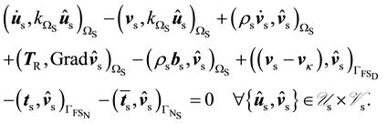 (47)
(47)
where
 is a constant over the solid domain with dimensions of mass per length cubed per time cubed to give our equations dimensional consistency. For the solids considered in this work, the first Piola-Kirchhoff stress
 uses the St. Venant-Kirchhoff strain tensor given in (10).
Problem 2 (Fluid sub-problem)
Find
 such that
 (48)
(48)
where
 and
and
 are as given in (5) and (6), and, for the linearly viscous, incompressible fluids considered in this work, the Cauchy stress
 is as given in (20).
Problem 3 (Mesh sub-problem)
Find
 such that
 (49)
(49)
Solving (49) using spatially constant material proper- ties
 and
and
 can can result in poor quality meshes if the solid displacement is large enough3. To prevent this, an artificial stiffness is imposed on the mesh, using
 and
and , in a manner such that it is stiffer near the interface and less stiff away from the interface. This propagates the distortion caused by the solid displacement throughout the entire mesh, instead of it being localized at the interface.
The global FSI problem is a direct sum of Problems 1, 2, and 3.
Problem 4 (Global FSI problem)
Find

such that (47), (48), and (49) are simultaneously satis- fied.
The individual sub-problems are coupled solely via the boundary conditions on the FSI interface . The glo- bally defined system in Problem 4 is a fully coupled non- linear system of equations. We have employed the New- ton-Raphson method to solve these equations, including all non-linear sub-problems that arise. We present some of the details in Appendix 9 since the calculations can be daunting, especially for the monolithic method.
5. FSI Algorithms
The numerical solution of Problem 4 is the focus of our study. We examine three different types of solution pro- cedures: partitioned, monolithic, and quasi-direct. These are often referred to as FSI coupling methods, although they can also be thought of as a family of algebraic solution methods to solve the fully coupled Problem 4.
3A poor quality mesh satisfies its boundary conditions but contains cells that are extremely distorted, such as cells with nearly parallel adjacent sides.
One of the key features of our study is that all three solution algorithms are implemented within the same software package (deal.ii). This feature allows us to use the same finite element assembly routines for all FSI coupling types, ensuring that computational cost differ- ences between the methods studied is not due to different implementations. Furthermore, the convergence criterion chosen are applied in exactly the same manner for each FSI algorithm, as described in Section 7.2.
The global solution procedure of the three coupling types is the same. After a setup procedure and applica- tion of initial conditions, a time loop advances the solu- tion with a prescribed time step size until the final simu- lation time is reached. For each time step, the three FSI coupling algorithms solve Problem 4 in different man- ners. We refer to the non-linear solution procedure within a single time step as FSI iterations.
5.1. Partitioned Coupling
The partitioned coupling method couples Problems 1, 2, and 3 in a sequential fashion to solve the global FSI problem. This coupling method is also referred to as Di- richlet-Neumann coupling, due to the way constraints are imposed on the FSI interface. There are other types of partitioned coupling, but we choose Dirchilet-Neumann coupling as it is by far the most common type used in practice: used by Turek et al. [2], Degroote et al. [6], Küttler et al. [23], and Campbell et al. [24], amongst many others. The FSI iterations for the partitioned me- thod involve solving the fluid, solving the solid, and solving the mesh; this process is iterated until conver- gence is attained. The partitioned algorithm is detailed in Figure 3(a).
We solve (48) with prescribed velocities on . As such, we enforce Dirichlet conditions on
 and define
 . The corresponding change to our finite dimensional vector spaces requires us to replace (39) and (44) with
 (50)
(50)
 (51)
(51)
respectively. The strong enforcement of the velocity coupling is achieved in our implementation through the use of deal.ii’s constraint tools [1]. Newton-Raphson iterations are used to solve the non-linear fluid sub- problem.
Once a fluid solution is obtained, Problem 1 is solved over the solid domain using the fluid traction as the driving force on the FSI interface. That is,
 and the applied traction on
 is computed as

(52)
which comes from (35) and (20). The function space definitions on
 do not need modification for the partitioned method. Due to the geometric non-linearities in Problem 1, a Newton-Raphson method is used to solve for the solid displacements and velocities.
If the change in position of
 is non-trivial (see Section 7.2 for discussion of this criterion), we deem it necessary to update the mesh position by solving Prob- lem 3. Before solving for the mesh displacement, it is well known [23] that the interfacial displacements should be under-relaxed to ensure convergence. The solid dis- placements and velocities are relaxed as
 (53)
(53)
 (54)
(54)
where the subscript
 denotes the iteration count and the superposed tilde denotes the non-relaxed solution from solving Problem 1. We find it beneficial (or, at a minimum, non-detrimental) to relax the entire solid solu- tion, rather than just the degrees of freedom whose sup- port is on
 .
.

Figure 3. Flowcharts demonstrating the partitioned (a); quasi-direct (b); and monolithic (c) FSI algorithms.
The scalar relaxation parameter
 can be chosen to be constant, but it has been shown [23] that allowing it to change between iterations can accelerate convergence. Aitken’s
 convergence acceleration method seems to be the most popular algorithm for choosing
 , and we have used it in this work. The position of the fluid-solid interface is viewed as a set of fixed points for the partitioned FSI iterations, and the secant method is used to extrapolate the expected position of the interface. The result is the recursive formula for computing the relaxa- tion factor
 (55)
(55)
and the discrete vector
 consists of the nodal values
from . The Euclidean inner product and norm are
used for the discrete vector. For the first FSI iteration of each timestep a relaxation factor of 0.75 is used.
Once the solid solution has been relaxed, we update the mesh displacements by solving Problem 3. The function space definitions (41) and (46) are augmented as
 (56)
(56)
 (57)
(57)
respectively, to account for enforcing a Dirichlet condi- tion on the fluid-structure interface. Unlike the fluid and solid sub-problems, the mesh motion is governed by a linear system of equations and only requires a single algebraic solve.
5.2. Quasi-Direct Coupling
The second algorithm of our study for quasi-direct coupling, as first performed by Tezduyar [25], is detailed
in Figure 3(b). The algorithm solves Problems 1 and 2 monolithically, and an iterative procedure is used to couple with Problem 3 to fully solve the complete FSI Problem 4. For each time step, we solve the coupled flu- id-solid system, update the mesh displacements, and ite- rate on these two solves until convergence is reached.
The quasi-direct algorithm does not use the Dirichlet- Neumann coupling scheme that the partitioned method uses. Rather, we construct a conforming velocity field over the entire reference domain
 as
as
 (58)
(58)
 (59)
(59)
The consequence of this choice is that (34) is strongly satisfied, which implies that
 (60)
(60)
after enforcing (35) and recognizing that the velocity weighting functions are chosen from the same function space. Another way to recognize that the tractions on
 do not contribute to the weak form is that
 and
and
 by construction of a conforming (conti- nuous) velocity space. Therefore, the traction continuity is implicitly satisfied and does not enter the quasi-direct (or monolithic) equations [26].
The solution from the fluid-solid does not need to be relaxed as it was for the partitioned algorithm. The relax- ation procedure is only used for iterative Dirichlet- Neumann coupling schemes for stability. Our only re- quirements on the mesh motion are the same as for the partitioned case. Namely,
 is computed using the function spaces given in (56) and (57).
5.3. Monolithic Coupling
The full monolithically coupled solution procedure is the third algorithm of our study and is detailed in Figure 3(c). Problem 4 is solved as a single non-linear system, with no FSI iterations necessary. We use the conforming velocity space given in (58) and (59) to strongly couple the fluid and solid domains.
The displacement fields
 and
and
 can be com- bined into a single conforming field, but doing so raises some computational challenges. Unlike the fluid-solid domains which are two-way coupled (they affect each other mutually), the solid-mesh displacement fields are one-way coupled. That is, solving Problem 3 for the mesh displacements should not directly influence the displacement field of the solid, while the solution of Problem 1 provides the driving boundary condition for the mesh solution. Thus, constructing a typical conform- ing finite element space over the entire domain has the detrimental affect of allowing the artificial mesh ‘stiff- ness’ to limit the motion of the solid structure.
We have used a simple and efficient method to strongly enforce (33) while avoiding the artificial stiff- ness phenomena. We solve Problem 4 using function spaces defined by (37), (40), (41), (42), (45), (46), (58), (59). The Newton-Raphson method is used to compute the solution, and we provide details of the linearization in the Appendix. Within each Newton-Raphson iteration, we weakly enforce the displacement continuity constraint within Problem 3. At the end of the iteration, the nodal mesh displacements on the interface are set to be equal to the solid displacement. In our numerical computations, we have found that weakly enforcing continuity yields mesh values that are relatively close to those computed for the solid. Also, modifying the mesh solution at the end of each Newton-Raphson iteration does not seem to affect the convergence characteristics of the method.
6. Code Verification
Verification of the discretized equations of motion, and the software in which it is implemented, is performed via the method of manufactured solutions (see, e.g., [27,28]). We perform the following sequence of analysis for the solid and fluid solvers separately: 1) choose an exact solution for the governing equations, 2) substitute this solution in the equations to obtain analytical expressions for the corresponding forcing functions and boundary conditions, 3) implement these into the code, and 4) compute an approximate solution. The error between the exact and approximate solutions is then computed according to some norm, and the process is repeated for a sequence of uniformly refined meshes.
Figure 4 shows the results of this process for several iterations of mesh refinement. The Figure 4(a) shows the individual components of the elastic displacement and velocity error declining as mesh size decreases, with a linear rate of
 under the
 norm when using bi-quadratic
 tensor-product elements for all fields. The Figure 4(b) shows the analogous situation for the velocity and pressure fields in the fluid solver, where the difference in convergence rate is due to the Taylor-Hood
 −
−
 tensor product elements used for the velocity and pressure, respectively.
Overall, this simple verification exercise demonstrates that the individual components of the FSI solver are functioning correctly. We will evaluate the correctness of the coupling implementation in the next section; more details regarding verification of the solvers can be found in Sheldon [29].
7. Model Validation
An FSI benchmark was proposed by Turek and Hron [2] for the purpose of facilitating comparison between dif- ferent FSI modeling approaches and algorithms, regard- less of coupling types or discretization schemes. This
 (a)
(a) (b)
(b)
Figure 4. Error convergence plots for the two-field elasticity formulation (a) and Navier-Stokes formulation (b). In each case, the expected rates of error convergence are achieved, with respect to the L2-norm. This demonstrates that each component of the FSI solver is functioning correctly.
benchmark consists of a numerical experiment involving laminar incompressible channel flow around a bluff body, which subsequently sheds vortical structures that excite a flexible tail until it reaches a state-state flow induced oscillation. Data were provided by Turek and Hron for the tip displacement of the elastic structure, hereafter called the flag (see Figure 5), and the drag and lift about the combined boundary of the flag and the cylinder to which the flag is attached. We used this benchmark as a means to validate the FSI model developed in this work, via direct comparison of our model’s predictions to that of Turek and Hron, and as a baseline for comparing the coupling strategies to one another.
7.1. Numerical Experiment Definition
The problem domain is depicted in Figure 5, where the channel, rigid cylinder, and elastic flag are noted. Flow is from left to right, with the cylinder slightly offset in the channel. Relevant dimensions are reproduced for the reader in Table 1. We will present our analysis of repro-

Figure 5. Turek and Hron [2] FSI benchmark domain with expanded view of cylinder and flag.

Table 1. Turek and Hron [2] FSI benchmark domain dimensions and material properties.
ducing the “FSI2” case of Turek and Hron, as it involves the largest structural deformations, and is therefore the most intense test for our solver. The material properties for this simulation are also reproduced for the reader in Table 1, where
 is the density,
 is the Possion’s ratio,
 is the viscosity,
 is the Young’s modulus, and
 is the mean inflow velocity. As before, the
 and
and
 subscripts indicate solid and fluid properties, respectively. Figure 6 shows an example of the flow field and solid deformation, using results from FSI2 after 16.5 simulation seconds, to help in visualizing the benchmark.
The boundaries of the computational domain are labeled in Figure 7, which also shows the mesh we used for our calculations. The boundary conditions are as follows: a parabolic fluid velocity inflow on :
:
 (61)
(61)
a no-slip fluid velocity on ,
,
 , and
, and :
:

Figure 6. Visualization of the velocity magnitude and flag deformation at t = 16:5 [s]. Solid displacement and fluid velocity are shown with their own color scales. The flag is shown as a wireframe to distinguish it from the fluid and the rigid cylinder.

Figure 7. Turek and Hron [2] FSI benchmark mesh with labeled boundaries and domains.
 (62)
(62)
a constant fluid pressure on , which is prescribed to be zero:
 (63)
(63)
a fixed solid displacement and velocity on :
:
 (64)
(64)
the interface conditions given in (33) and (34) on , and the mesh displacement condition given in (29) on
 ,
,
 ,
,
 ,
,
 , and
, and .
.
All fields are initially zero. For the first two seconds the fluid inlet velocity is subject to a smooth increase defined by
 (65)
(65)
A timestep size
 was used in all cases to satisfy the Courant-Friedrichs-Lewy (CFL) condition [30], computed from a maximum flow velocity and minimum cell diameter of approximately
 and
and , respectively.
As in Section 6, all subsequent results in the section were computed with
 elements for the solid dis- placement and velocity, Taylor-Hood
 −
−
 ele- ments for the fluid velocity/pressure,
 elements for the mesh displacement, and the Crank-Nicholson method for the time discretization. For consistency in comparison of the timing results, all simulations were performed on the same computer. Linear algebraic solves were done with the sparse direct solver UMFPACK [31].
7.2. Convergence Criterion
The FSI coupling strategies that we have employed in this work all require some sort of sub-iteration at each time step in the simulation process. For the partitioned schemes, we make fixed-point iterations between the solver components to converge the solution, while for the monolithic approaches we use Newton-Raphson itera- tions. Consistency in defining convergence criteria for the global coupled FSI solution, that is applicable to both the partitioned and monolithic approaches, is a key point of this work. If this metric is not chosen consistently, we will not be able to say that the solutions are similarly converged to the same level of error, and therefore be unable to make comparisons regarding the wall clock time.
For the global FSI solution, the convergence criterion [23,32] is given by
 (66)
(66)
where
 and
and
 refer to the solid displacement at the current and previous FSI iteration, whether that iteration is fixed-point (partitioned) or Newton-Raphson
(monolithic). Here,
 is the standard
 norm
norm
over the fluid-solid interface, and
 is some convergence tolerance, which we typically defined to be
 E−10, for all coupling methods. For the partitioned method, we perform this solution check after every instance where the solid displacement is solved, while for the monolithic approaches, we perform this check after each Newton Iteration. In all coupling approaches, once this criterion is satisfied, we exit the sub-iteration loop and move on to the next time step.
7.3. Computations
In Turek and Hron’s FSI2 simulation benchmark, the system starts at rest and the speed of the inflow grows until it levels off to some steady value. After this initial transient period, which is approximately the first twelve seconds of simulation time, the solution reaches a steady state of oscillation. All results over a given periodic interval after this time are interchangeable, and as such we have normalized the comparison time interval on all forthcoming images.
We were able to reproduce the results given by Turek and Hron, for the x- and y-displacement of point A, at the mid-point of the tip of the tail, and the lift and drag gen- erated about the combined surface of the flag and cylind- er. Our calculations are nearly indistinguishable whether using the partitioned, quasi-direct, or monolithic coupl- ing, as seen in Figures 8 and 9. Table 2 provides nu- merical values for the maximum and minimum of the displacement, drag, and lift from both Turek and Hron’s work and our own, along with the percent error between our solutions and the validation data. The maximum deviation from the validation data for any quantity is 4%, with the three coupling methods each being the most accurate for some quantities and the least for others. Overall, the visual and numerical results demonstrate the coupling methods are all within an acceptable deviation from the validation data, and can be confirmed to func- tioning correctly. Even more so, we have demonstrated that using the same convergence criterion for the global FSI problem has resulted in three solutions that are quite similar to each other.
Finally, Figure 10 plots the wall clock runtime of the three coupling techniques over 20 seconds of simulation time. The noticeable change in slopes at approximately 7 simulation seconds aligns with the time at which the flag
 (a)
(a) (b)
(b)
Figure 8. The x- and y-displacement of point A on the flag tip. Our monolithic and quasi-direct schemes show nearly identical results to Turek and Hron [2], while our partitioned scheme is slightly different.
Table 2. Maximum and minimum values for the x- and y-displacements of point A, and the lift and drag generated about the combined surface of the flag and cylinder. The results from Turek and Hron [2] are presented alongside ours, and our per- cent error from theirs is calculated.
 (a)
(a) (b)
(b)
Figure 9. The drag and lift generated about the combined surface of the flag and cylinder. All three of our schemes show larger minimum values than Turek and Hron [2] do when calculating the drag, with otherwise good agreement. Our monolithic and quasi-direct schemes capture the com- plex shape of of Turek and Hron’s lift results [2], while our partitioned scheme matches the global maximum and minimum values but not all local the minimums and max- imums in-between.

Figure 10. Time study for partitioned, quasi-direct, and monolithic coupling over 20 simulation seconds (8000 timesteps). Our partitioned coupling scheme required over twice the amount of CPU time per time step compared to our quasi-direct coupling scheme, which in turn required approximately twice that of our monolithic coupling scheme.
oscillations began to be significant, thus requiring more sub-iterations of the FSI algorithm. As can be seen, for this benchmark case the partitioned scheme requires over twice the amount of CPU time to solve any given time- step compared to the quasi-direct scheme, and the mono- lithic scheme requires even less CPU time than that. Given that we have held each solver to the same conver- gence criterion, and given that all other aspects of the simulation are held constant, we can state that for this problem, the monolithic scheme is certainly more effi- cient.
8. Summary and Conclusions
A methodology has been presented for comparing FSI coupling algorithms in the most fair and unbiased man- ner we could conceive. We developed a numerical ALE framework that allows for different FSI coupling algo- rithms to be evaluated for accuracy and efficiency in a quantitative manner. By holding constant many of the usually confounding factors, such as the grid, mesh mo- tion, discretization approach, and solver tolerances, we were able to compare three different coupling strategies. These include a Dirichlet-Neumann partitioned coupling method, a monolithic coupling method, and quasi-direct coupling method. Each of these is tightly-coupled and uses the same convergence criterion to define when the global FSI solution is converged during a given time step. All three coupling methods use the same software infrastructure, system of equations assembly code, algebraic solver, and parameters. Other than their inherent differences in methodology, they are identical.
The benchmark proposed by Turek and Hron [2] was used to test the FSI coupling strategies developed in this work. We were able to achieve results which accurately reproduce those provided by Turek and Hron to within four percent at worst, generally within two percent. For this case, our results show that monolithic coupling and quasi-direct coupling are slightly more accurate, with respect to the validation data, than partitioned coupling and slightly better at capturing fine details along the in- terface. We also found that monolithic coupling and qua- si-direct coupling are significantly faster than partitioned coupling when held to tight coupling tolerances. This substantiates Michler’s hypothesis discussed earlier, that monolithic schemes can outperform partitioned schemes when held to the same tolerances [9], at least for the spe- cific problem consider herein.
While this work aims to present a methodology for proper comparison between ALE FSI coupling algo- rithms, we acknowledge that the benchmark example considered is neither exhaustive nor addresses many of the other practical simulation issues. In the weak-coupl- ing limit, we might expect that a partitioned or quasi- direct approach would be more efficient than a mono- lithic approach. Large three-dimensional problems may also change the comparison results: as the number of degrees of freedom grows quickly, the cost of solving a large linear system becomes the main computational cost and scalability needs to be addressed. The choice of li- near algebraic solvers could also greatly sway the study, as extremely efficient methods for solving each subprob- lem exist, but cannot be applied to the monolithic system of equations. The governing equations and the choice of discretization scheme will also undoubtedly affect any sort of computational cost comparisons. Finally, there exist numerous other ALE partitioned coupling methods (e.g. Robin-Robin coupling rather than Dirichlet-Neu- mann) that may be more accurate and efficient than the methods we investigated. These aspects of the ALE FSI solution can be studied within our numerical framework, and we leave them as future research efforts.
Acknsowledgements
J. Sheldon gratefully acknowledges financial support from Naval Sea Systems Command, Advanced Subma- rine Systems Development Office (SEA 073R) with Ms. Diane Segelhorst and Mr. Patrick Tyler as program ma- nagers. S. Miller and J. Pitt acknowledge internal support for this research from the Applied Research La- boratory at The Pennsylvania State University.
REFERENCES
[1] W. Bangerth, T. Heister and G. Kanschat, “Deal. II Differential Equations Analysis Library,” Technical Reference. http://www.dealii.org
[2] S. Turek and J. Hron, “Proposal for Numerical Benchmarking of Fluid-Structure Interaction between an Elastic Object and Laminar Incompressible Flow,” Fluid- Structure Interaction, 2006, pp. 371-385.
[3] T. Wick, “Fluid-Structure Interactions Using Different Mesh Motion Techniques,” Computers & Structures, Vol. 89, No. 13, 2011, pp. 1456-1467. http://dx.doi.org/10.1016/j.compstruc.2011.02.019
[4] H. G. Matthies and J. Steindorf, “Partitioned but Strongly Coupled Iteration Schemes for Nonlinear Fluid-Structure Interaction,” Computers & Structures, Vol. 80, No. 27, 2002, pp. 1991-1999. http://dx.doi.org/10.1016/S0045-7949(02)00259-6
[5] C. F¨orster, W. A. Wall and E. Ramm, “Artificial Added Mass Instabilities in Sequential Staggered Coupling of Nonlinear Structures and Incompressible Viscous Flows,” Computer Methods in Applied Mechanics and Engineering, Vol. 196, No. 7, 2007, pp. 1278-1293. http://dx.doi.org/10.1016/j.cma.2006.09.002
[6] J. Degroote, K. Bathe and J. Vierendeels, “Performance of a New Partitioned Procedure versus a Monolithic Procedure in Fluid-Structure Interaction,” Computers & Structures, Vol. 87, No. 11, 2009, pp. 793-801. http://dx.doi.org/10.1016/j.compstruc.2008.11.013
[7] G. Hou, J. Wang and A. Layton, “Numerical Methods for Fluid-Structure Interaction―A Review,” Communications in Computational Physics, Vol. 12, No. 2, 2012, pp. 337-377.
[8] M. Heil, “An Efficient Solver for the Fully Coupled Solution of Large-Displacement Fluid-Structure Interaction Problems,” Computer Methods in Applied Mechanics and Engineering, Vol. 193, No.1-2, 2004, pp. 1-23. http://dx.doi.org/10.1016/j.cma.2003.09.006
[9] C. Michler, “A Monolithic Approach to Fluid-Structure Interaction,” Computers & Fluids, Vol. 33, No. 5-6, 2004, pp. 839-848. http://dx.doi.org/10.1016/j.compfluid.2003.06.006
[10] ADINA, “Adina fsi,” Cited 08-23-2012.
[11] M. Heil and A. Hazel, “Oomph-lib,” Cited 09-12-2012.
[12] M. Gurtin, E. Fried and L. Anand, “The mechanics and Thermodynamics of Continua,” Cambridge University Press, 2009.
[13] R. Bowen, “Introduction to Continuum Mechanics for Engineers,” Plenum Press, New York, 1989. http://dx.doi.org/10.1007/978-1-4684-7761-0
[14] P. Chadwick, Continuum Mechanics: Concise Theory and problems. Dover Publications, 1999.
[15] A. Spencer, “Continuum mechanics,” Dover Publications, 2004.
[16] T. Tezduyar, K. Takizawa, C. Moorman, S. Wright, and J. Christopher, “Space-Time Finite Element Computation of Complex Fluid-Structure Interactions,” International Journal for Numerical Methods in Fluids, Vol. 64, No. 10-12, 2010, pp. 1201-1218. http://dx.doi.org/10.1002/fld.2221
[17] Y. Bazilevs, K. Takizawa and T. E. Tezduyar, “Computational Fluid-Structure Interaction: Methods and Applications,” Wiley, New York, 2012.
[18] C. Peskin, “The Immersed Boundary Method,” Acta Numerica, Vol. 11, 2002, pp. 479-517.
[19] M. Uhlmann, “An Immersed Boundary Method with Direct Forcing for the Simulation of Particulate Flows,” Journal of Computational Physics, Vol. 209, No. 2, 2005, pp. 448-476. http://dx.doi.org/10.1016/j.jcp.2005.03.017
[20] J. Hron and S. Turek, “A Monolithic Fem/Multigrid Solver for an Ale Formulation of Fluid-Structure Interaction with Applications in Biomechanics,” Fluid-Structure Interaction, Vol. 53, 2006, pp. 146-170.
[21] T. Richter and T. Wick, “Finite Elements for Fluid- Structure Interaction in Ale and Fully Eulerian Coordi- nates,” Computer Methods in Applied Mechanics and En- gineering, Vol. 199, No. 41, 2010, pp. 2633-2642. http://dx.doi.org/10.1016/j.cma.2010.04.016
[22] M. P. Robert Cook, David Malkus and R. Witt, “Concepts and Applications of Finite Element Analysis,” JohnWiley & Sons, 4 Edition, 2001.
[23] U. Kuttler and W. A. Wall, “Fixed-Point Fluid-Structure Interaction Solvers with Dynamic Relaxation,” Computational Mechanics, Vol. 43, No. 1, 2008, pp. 61-72. http://dx.doi.org/10.1007/s00466-008-0255-5
[24] R. Campbell and E. Paterson, “Fluid-Structure Interaction Analysis of Flexible Turbomachinery,” Ph.D. Thesis, The Pennsylvania State University, 2011.
[25] T. E. Tezduyar, S. Sathe, R. Keedy and K. Stein, “Space- Time Finite Element Techniques for Computation of Fluid-Structure Interactions,” Computer Methods in Applied Mechanics and Engineering, Vol. 195, No. 17, 2006, pp. 2002-2027. http://dx.doi.org/10.1016/j.cma.2004.09.014
[26] S. Kang, H. Choi and J. Yoo, “Investigation of Fluid- Structure Interactions Using a Velocity-Linked p2/p1 Finite Element Method and the Generalized-A Method,” International Journal for Numerical Methods in Engineering, Vol. 90, No. 12, 2012, p. 1529.
[27] C. Roy, C. Nelson, T. Smith and C. Ober, “Verification of Euler/Navier-Stokes Codes Using the Method of Manu- factured Solutions,” International Journal for Numerical Methods in Fluids, Vol. 44, No. 6, 2004, pp. 599-620. http://dx.doi.org/10.1002/fld.660
[28] P. J. Roach, “Code Verification by the Method of Manu- factured Solutions,” Journal of Fluids Engineering- Transactions of the ASME, Vol. 124, No. 1, 2002, pp. 4-10.
[29] J. Sheldon, “A Comparison of Fluid-Structure Interaction Coupling Algorithms Using the Finite Element Method,” Master’s Thesis, The Pennsylvania State University, 2012.
[30] S. Osher and R. Fedkiw, “Level Set Methods and Dynamic Implicit Surfaces,” Springer, New York, 2003.
[31] T. Davis, “Algorithm 832: Umfpack v4. 3-An unsymmetric-pattern multifrontal method,” ACM Transactions on Mathematical Software (TOMS), Vol. 30, No. 2, 2004, pp. 196-199. http://dx.doi.org/10.1145/992200.992206
[32] S. Deparis, M. A. Fern´andez and L. Formaggia, “Acceleration of a Fixed Point Algorithm for Fluid-Structure Interaction Using Transpiration Conditions,” ESAIM: Mathematical Modelling and Numerical Analysis, Vol. 37, No. 4, 2003, pp. 601-616.
Appendix
Linearization
Problems 1, 2, and 4 are non-linear systems of equations which we have chosen to solve numerically via the Newton-Raphson (NR) method. Problem 3 is linear, but we formulate the solution via the NR method for consis- tency. For the partitioned and quasi-direct algorithms, the mesh solution is obtained with a single NR iteration. Given an initial solution estimate (computed from the previous time step or initial conditions) iterate over the following problem until convergence is reached:
Problem 5 (Newton-Raphson iterate)
Given a solution vector , compute
 via
via
 (67)
(67)
where the vector
 is the residual vector,
 is the Jacobian matrix, and
 is the solution update vector.
The solution and residual vectors are
 (68)
(68)
The sub-vectors within
 correspond to the nodal values of the solid, fluid, and mesh component blocks of the solution. The individual components of the residual
vector are
 (69)
(69)
 (70)
(70)
 (71)
(71)
 (72)
(72)
 (73)
(73)
The Jacobian matrix is formed by taking the the derivative of the residual vector with respect to the nodal unknowns:
 (74)
(74)
In the most general form, the discrete equations for the monolithic system are written as
 (75)
(75)
Although this system seems daunting, application of the residual vector components, from (69), (70), (71), (72), and (73), to the Jacobian definition in (74) shows that many of the terms are zero for all coupling algorithms, reducing the system to
 (76)
(76)
Discrete Monolithic Equations
When discretized monolithically, (76) is further simplified due to the conforming velocity fields given in (58) and (59). As shown in (60), these velocity fields
lead to the tractions on the fluid-solid interface not contributing to the monolithic (or quasi-direct) equations.
This eliminates ,
,
 ,
,
 , and
, and
 from
from
(76), resulting in
 (77)
(77)
where the terms marked by
 arise due to the con- forming velocity space in (58).
Discrete Quasi-Direct Equations
The quasi-direct discretization of (76) is similar to the monolithic discretization in that the tractions do not con- tribute on the interface. This results in the same terms being eliminated as were in the monolithic case. Fur- thermore, as the quasi-direct approach only solves Prob- lems 1 and 2 monolithically, and iterates their solution with that of Problem 3, (76) can be separated into two smaller systems which reflect the coupled fluid-solid and seperate mesh:
 (78)
(78)
 (79)
(79)
Discrete Partitioned Equations
With partitioned coupling, Problems 1, 2, and 3 are all solved sequentially. This allows for (76) to be simplified into three independent smaller systems for the solid, fluid, and mesh:
 (80)
(80)
 (81) (82)
Jacobian Component Calculations
The actual Jacobian calculations are simply derivatives of the residuals presented previously, and so they have been ommited. When evaluating the Jacobians, the fol- lowing tensor calculus identities from Gurtin [12] are useful:
 (83)
(83)
 (84)
(84)
 (85)
(85)
In our calculations, we approximate the mesh (fluid domain) velocity within each time step as
 (86)
(86)
Because it is not one of our primitive variables.