Atmospheric and Climate Sciences
Vol.3 No.4(2013), Article ID:36236,10 pages DOI:10.4236/acs.2013.34045
Southern and Tropical Indian Ocean SST: A Possible Predictor of Winter Monsoon Rainfall over South India
1Centre for Ocean-Land-Atmosphere Studies, Calverton, USA
2K. Banerjee Center of Atmospheric & Ocean Studies, Institute of Interdisciplinary Studies, University of Allahabad, Allahabad, India
Email: *ravis@cola.iges.org
Copyright © 2013 Ravi P. Shukla et al. This is an open access article distributed under the Creative Commons Attribution License, which permits unrestricted use, distribution, and reproduction in any medium, provided the original work is properly cited.
Received April 23, 2013; revised May 25, 2013; accepted July 1, 2013
Keywords: Winter Monsoon Rainfall over South India; Southern/Tropical Indian Ocean; Multivariate/Linear Regression Models
ABSTRACT
The complexities in the relationship between winter monsoon rainfall (WMR) over South India and Sea Surface temperature (SST) variability in the southern and tropical Indian Ocean (STIO) are evaluated statistically. The data of the time period of our study (1950-2003) have been divided exactly in two halves to identify predictors. Correlation analysis is done to see the effect of STIO SST variability on winter monsoon rainfall index (WMRI) for South India with a lead-lag of 8 seasons (two years). The significant positive correlation is found between Southern Indian Ocean (SIO) SST and WMRI in July-August-September season having a lag of one season. The SST of the SIO, Bay of Bengal and North Equatorial Indian Ocean are negatively correlated with WMRI at five, six and seven seasons before the onset of winter monsoon. The maximum positive correlation of 0.61 is found from the region south of 500 S having a lag of one season and the negative correlations of 0.60, 0.53 and 0.57 are found with the SST of the regions SIO, Bay of Bengal and North Equatorial Ocean having lags of five, six and seven seasons respectively and these correlation coefficients have confidence level of 99%. Based on the correlation analysis, we defined Antarctic Circumpolar Current Index A and B (ACCIA (A) & ACCIB (B)), Bay of Bengal index (BOBI (C)) and North Equatorial Index (NEI (D)) by averageing SST for the regions having maximum correlation (positive or negative) with WMRI index. These SST indices are used to predict the WMRI using linear and multivariate linear regression models. In addition, we also attempted to detect a dynamic link for the predictability of WMRI using Nino 3.4 index. The predictive skill of these indices is tested by error analysis and Willmott’s index.
1. Introduction
Indian summer monsoon, which is a part of the Asian monsoon system, is a regular annual phenomenon which brings heavy rainfall to India and adjacent countries during summer monsoon season (June to September; JJAS). It contributes about 70% - 90% of rainfall in most parts of country whereas, the rainfall during October-November-December (OND) over south India which is commonly referred as winter monsoon rainfall. It contributes about 50% of annual rainfall in the east cost of Indian Peninsula. The winter monsoon is highly variable both spatially and temporally. During winter monsoon season the prevailing wind becomes north-easterly and the zone of maximum rainfall migrates to southern India and Sri Lanka. Over the years, there are many instances of the years with flood (strong monsoon) or drought (weak monsoon) during which South India as a whole receives excess or deficient seasonal rainfall, respectively [1]. In an agricultural country like India, the success or failure of the summer/winter monsoon and its effects on agricultural production and water scarcity on regional basis are always of great concern. Even small fluctuation in the seasonal rainfall can have devastating impacts on agricultural sector. Winter monsoon rainfall (WMR) is comprised of five meteorological subdivisions namely Coastal Andhra Pradesh (CAP), Tamilnadu (TAM), Kerala (KER), South Interior Karnataka (SIK) and Rayalaseema (RAY) of South India. The water received during the winter monsoon season is utilized for various purposes viz, hydroelectric power production, irrigation of farm lands and drinking water in these subdivisions. Hence, the amount of rainfall during winter season over South India is very significant. Accurate long range prediction of winter monsoon rainfall can improve planning to mitigate the adverse impacts of rainfall variability and will be beneficial to policy makers and farmers both.
Further, many researchers have studied the predictability/trends of the Indian summer monsoon [2-16] using dynamical as well as statistical models. For more than one century, the prediction of Indian Monsoon Rainfall has been based on empirical models [2,3,17-21]. The prediction and predictability of WMR is still in early stage in spite of its potential societal and economical impact for South India. There are few studies which try to predict WMR using India ocean dipole index, Southern oscillation Index [22-27] and applying statistical technique.
Gradients of Sea Surface Temperature (SST) are important in determining the position of precipitation over the tropics including monsoon regions. It is assumed that the SST Anomaly (SSTA) over Indian Ocean vitally determines the monsoon rainfall variability. Shukla and Fennessy [28] pointed out that the annual cycle of SST in the Indian Ocean is significant in establishing the monsoon circulation and rainfall using General Circulation Model (GCM). The association of WMR on global climate including ENSO and Indian Ocean SST is still in early stage. Influence of ENSO and IOD on WMR has been investigated by Bhanu Kumar et al. [29] and interesting relationships were traced out. Kripalani and Kumar [30] extended the study between the northwest monsoon rainfall and IOD. Furthermore, an influence of monsoon upper-air temperatures over India on WMR was thoroughly studied by Bhanu Kumar et al. [31]. In all the above studies related to WMR, no attempt was made to understand the effect of sea Surface temperature variability in the Southern as well as tropical Indian Ocean (STIO) on the WMR monsoon on lead-lag of 8 seasons (2 years).
In the present study, attempt has been made to understand the Indian Ocean SST variability over STIO region with WMRI for 53 years (1950-2003) of extended Reynolds Smith reconstructed version 2 data [32]. The quality of the Reynolds SST version 1.0 data was very poor in southern ocean region (below 50˚S) but version 2.0 has improved much due to the inclusion of new schemes.
The variability of STIO SST and WMRI relationship is examined under the lead-lag time scales of 08 seasons for providing some insight into the possibility of early prediction of winter monsoon rainfall. This relationship will enable us to understand dependency of winter monsoon conditions on Southern Indian Ocean (SIO) SSTA, and in turn will provide important clues to oceanic system memory, which is still poorly understood.
Correlation analysis is done to see the effect of STIO SST and Niño-3.4 index [33,34] on WMR with a lead-lag of 8 seasons. Based on this analysis, we have defined SST index of those seasons which have confidence level of more than 99%. The regression and multiple regression technique have been used to study the predictability of the WMRI with above indices individually as well as in various combinations.
2. Data Used
The winter monsoon rainfall amounts for 5 meteorological subdivisions namely CAP, RAY, TAM, SIK and KER have been collected from the Indian Institute of Tropical Meteorology (IITM) website for the period 1950-2003. The mean of these meteorological subdivisions have computed and termed as Winter Monsoon Rainfall index over South India.
The extended reconstructed SST (ERSST, version 2.0, 2˚ ´ 2˚ resolutions) is used in the present study, which employs improved high frequency analysis and error analysis, use to sea ice to SST conversion algorithm and adjustment of the bias correction [32]. This data set contains global record of monthly SST from 1871 to 2003 but due to the uncertainties and data scarcity in the earlier data set of 19th century the temporal coverage has been considered only from 1949 to 2003.
3. Results and Discussion
3.1. Correlation Analysis between STIO SST and Winter Monsoon Rainfall Index (WMRI)
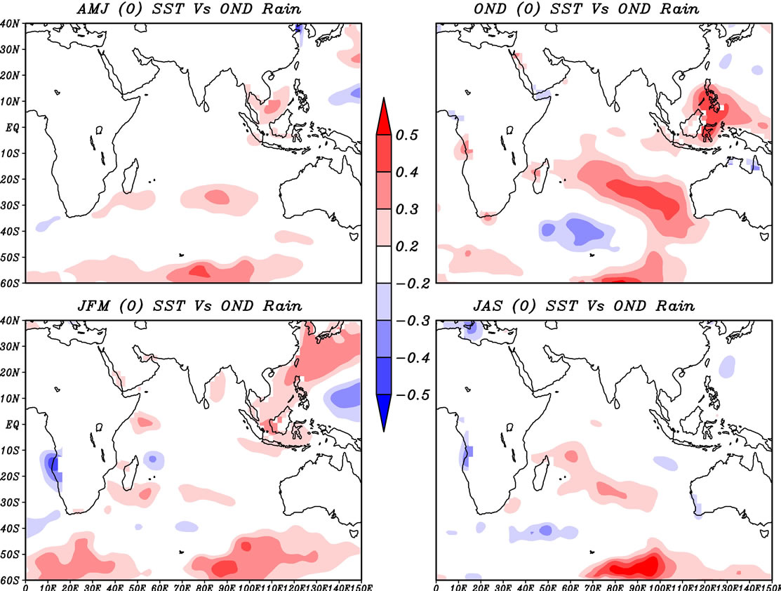
The correlation coefficients between SST variability in the STIO region for the seasons January-March (JFM), April-June (AMJ), July-September (JAS), and OctoberDecember (OND) with WMRI have been computed and presented in Figure 1 with a lead-lag of 0 - 7 seasons. We have used the leading correlation of WMRI up to 2 years which will enable us to study the long-term effect of STIO SST on winter monsoon. Positive correlation between STIO SST in JAS season with a lead of one season w.r.t. WMRI is found in Figure 1(a) having a maximum value of 0.61 which is significant above 99% confidence level near 90˚E, 55˚S. The positive significant correlations are similar for the region 50˚S to 60˚S by leading SST for 2 (AMJ) and 3 (JFM) seasons respectively. We have extended our analysis by leading SST with respect to WMRI for more than a year. The interesting finding is that the correlations for the domain of our study are negative by leading SST more than a year. The correlations are found to be low for most of the domain although significant at few scattered places by lagging SST for 2 to 5 seasons in the STIO region. For JAS season (6 season before onset the winter monsoon) (Figure 1(b)), the negative correlation value reaches a maximum of −0.5 with a confidence level of 99% near 50˚S and 110˚E (Figure 1(b)). For AMJ and JFM (7 and
 (a)
(a) (b)
(b)
Figure 1. (a) (b) Correlation coefficient (r) between sea surface temperature (SST) variability in the Southern/Tropical Indian Ocean (STIO) and Winter Monsoon Rainfall Index (WMRI) over South India lead-lag by 1 - 8 season(s) (The quantity in bracket indicates the lead-lag in years).
8 seasons before the onset of the monsoon), negative correlation is high over Bay of Bengal and near southern tip of India respectively. The correlation between Nino 3.4 index and WMRI with a lead lag of 8 seasons have been computed and shown in Figure 2. It is found that Nino 3.4 index with a lead of 2 - 3 season have a positive correlation of 0.29 and 0.24 respectively whereas a negative correlation of 0.49 has been found with a lead of 7 seasons.
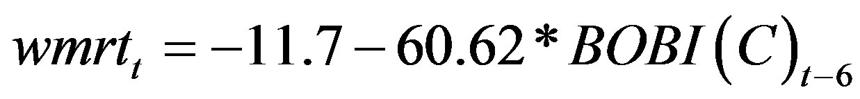
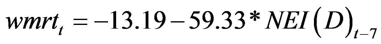
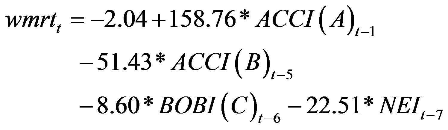
Based on the correlation analysis we have selected predictors by taking area averaged SST anomaly for the regions having highest positive or negative correlations and is tabulated in Table 1. The indices, defined thus are ACCIA (A), ACCI B (B), BOBI (C) and NEI (D) and were correlated with WMRI shown in Figures 3(a)-(d) and its value is 0.61, −0.60, −0.53 and −0.57 respectively.
Figure 2 shows the correlation coefficients of the Niño 3.4 index with WMRI. The following predictor has been found to have a correlation with the WMRI for period 1950-1976 with a confidence level of 99%: Niño3.4 index (seven seasons before onset of Monsoon) and its value is −0.49 (Figure 3(e)).
3.2. Regression Models for the Present Study
Different regression models [35] have been constructed for predicting the WMRI with different predictors. Following regression equations have been obtained:
 (1)
(1)
 (2)
(2)
 (3)
(3)
 (4)
(4)
 (5)
(5)
 (6)
(6)
 (7)
(7)
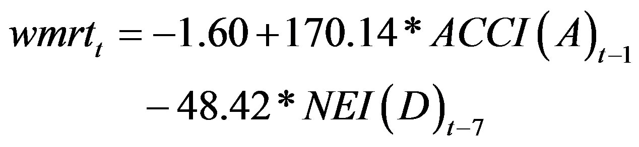
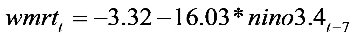
where wmrit = WMRI index at time t
ACCI(A)t–1 = ACCI (A) index 1 seasons earlier ACCI(B)t–5 = ACCI (B) index 5 seasons earlier BOBI(C)t–6 = BOBI (C) index 6 seasons earlier NEI(D)t–7 = NEI (D) index 7 seasons earlier nino3.4t–7 = nino3.4 index 7 seasons earlier Overall, seven regression models have been developed. Five regression models for individual predictors and two multiple regression models. 27 patterns were used in the
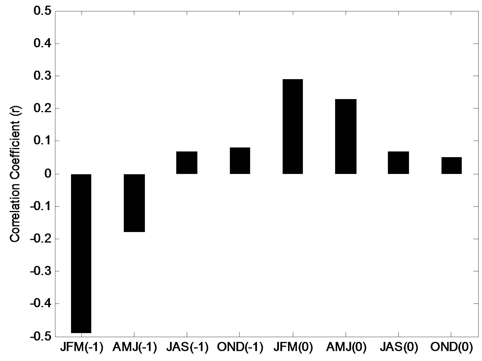
Figure 2. Correlation coefficient (r) between Nino 3.4 index and WMRI over South India lead-lag by 1-8 season(s).
training set for the determination of coefficients and 27 were used for the evaluation of model on unseen patterns (predicated set). The skills of these regression models have been evaluated using the root mean square error (RMSE), correlation coefficient (r) and Willmott’s index (WI) with the observed precipitation. The standard deviation (SD) of the observed and predicted precipitation has also been analysed. The categorical forecast skill measures e.g. accuracy, bias, probability of detection (POD), probability of false detection (POFD) and threat score (TS) are also calculated for each prediction. These skill score measures the fraction of observed and/or forecast events that were correctly predicted.
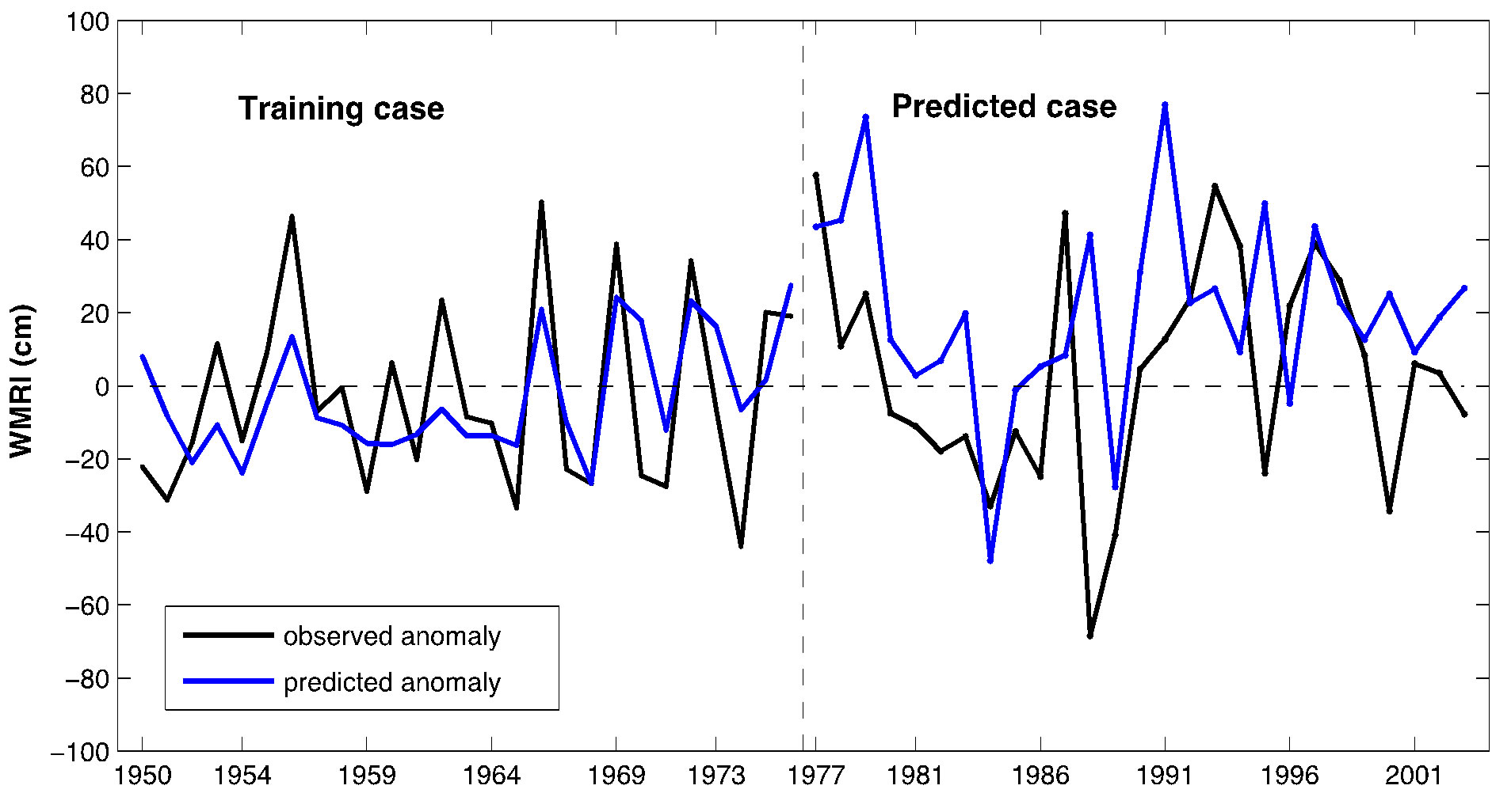
Figure 4 shows the comparison of model output WMRI with observed WMRI in training and test case for regression models A (Figure 4(a)), B (Figure 4(b)), C (Figure 4(c)), D(Figure 4(d)), multiple regression models A + B + C + D (Figure 4(e)), A + B (Figure 4(f)) and Nino 3.4t–7 regression model (Figure 4(g)).
Table 2 summarises the prediction skills of these models for the training and test cases both. It can be seen that for training case all the regression models, the RMSE is smaller than the SD of the observed data (26.15) implying that all regression models give prediction better than the mean (Table 2). SD of all regression models is less than observed SD for training case and the correlation coefficients are high for each regression model. For prediction case, it can been seen that none of the regression models have RMSE smaller than the SD of observed data (30.93) implying that none of the regression models give prediction better than the mean in case of prediction case but correlation coefficients are significant for ACCIA (A), NEI (D) and A + D regression model.
Figure 5 shows the comparison of model output with observations for prediction case. It may be noted that there were three El-Nino years in the period of our study viz, 1982, 1991 and 1997 and three La-Nina years viz, 1988, 1995 and 1998. A + D multiple regression model captures same sign of 4 ENSO years (1982, 1991, 1997,
 (a)
(a)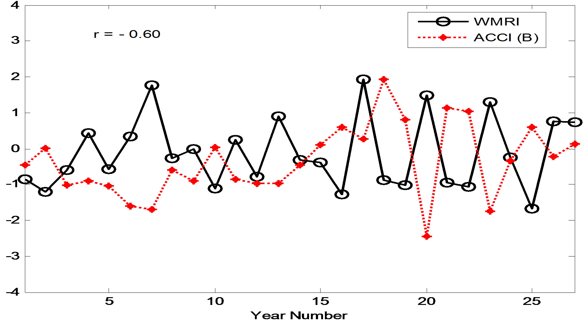 (b)
(b) (c)
(c)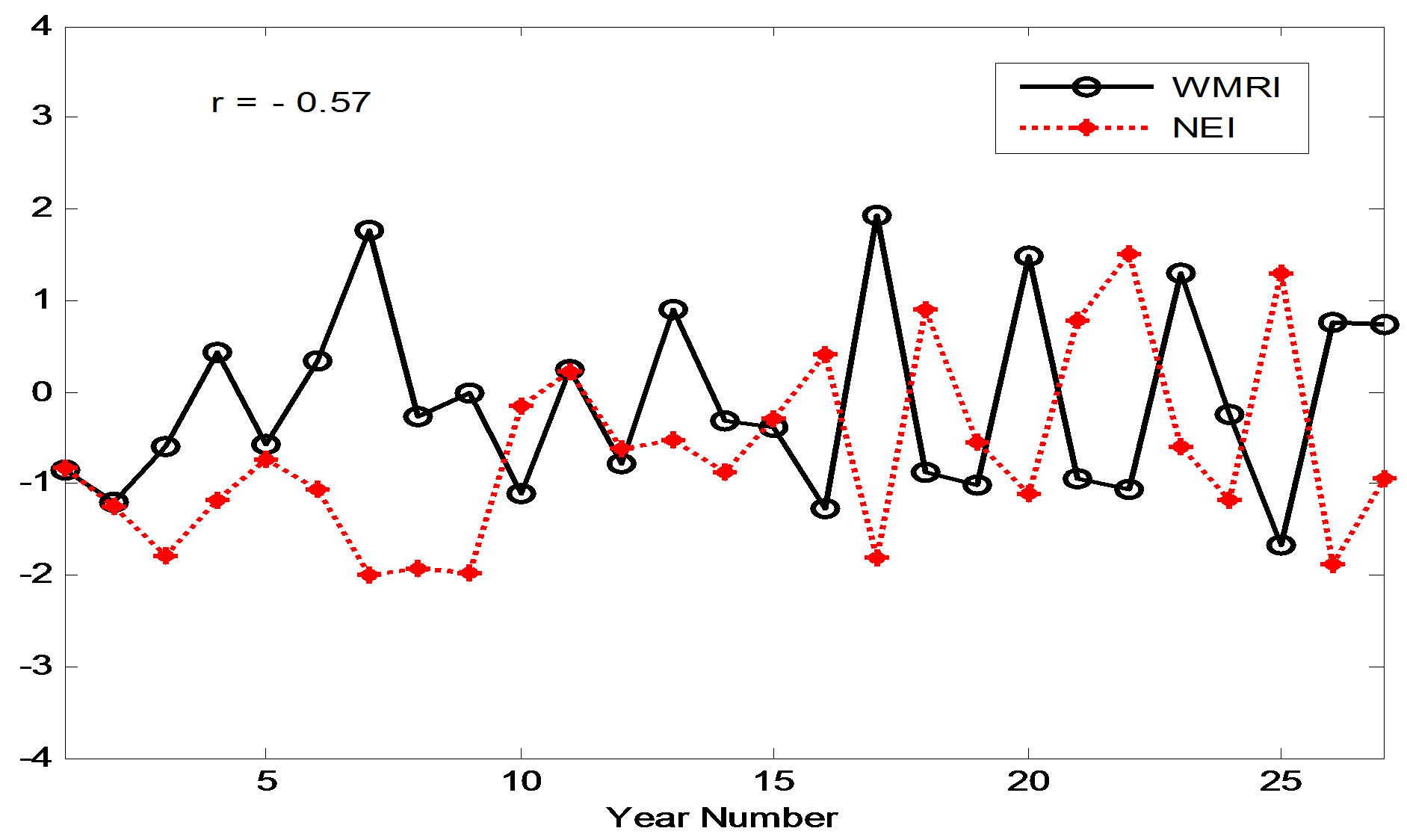 (d)
(d) (e)
(e)
Figure 3. (a)-(e) Time series of observed WMRI normalized anomaly (solid black line) and (a) Antarctic Circumpolar Current Index A (ACCI (A)) with a lag of 1 season (July-August-September), (b) Antarctic Circumpolar Current Index B (ACCI (B)) with a lag of 5 (July-August-September) season, (c) Bay of Bengal index (BOBI (C)) with lag of 6 (April-May-June) season, (d) North Equatorial Index (NEI (D)) with lag of 7 (January-February-March) season before the onset of monsoon (dashed red line) and (e) Niño 3.4 index with a lag of 7 seasons (dashed red line).
1998) and ACCI (A) regression model and Nino 3.4t–7 regression models also capture the same sign for three ENSO years.
3.3. Willmott’s Index (WI)
To test the results statistically, we also calculated the Willmott’s Index (WI) for regression as well as multiple regression model. The Willmott’s index (WI) is given by [36]
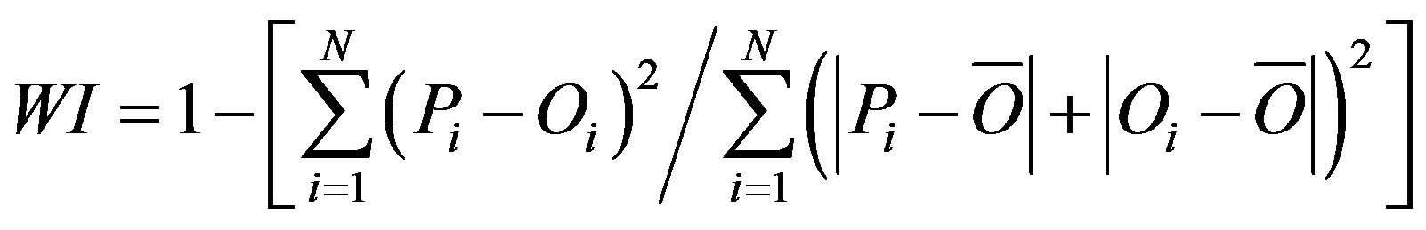
where,  ,
,  and
and  denote the observed value in the ith case, predicted value in ith case, and mean observed value respectively.
Wilmott [36] proposed Wilmott’s index of agreement (WI) and is widely used [37,38]. The value WI is dimensionless and varies between 0 and 1 which is a measure of the degree to which models predictions are error free when compared with the observations [36,39].
The WI has been computed and shown in Table 3, it is clear that A + B + C + D multiple regression model, A + D multiple regression model, ACCI (A) regression model and NEI (D) regression model have WI value 0.89, 0.86,
 (a)
(a) (b)
(b)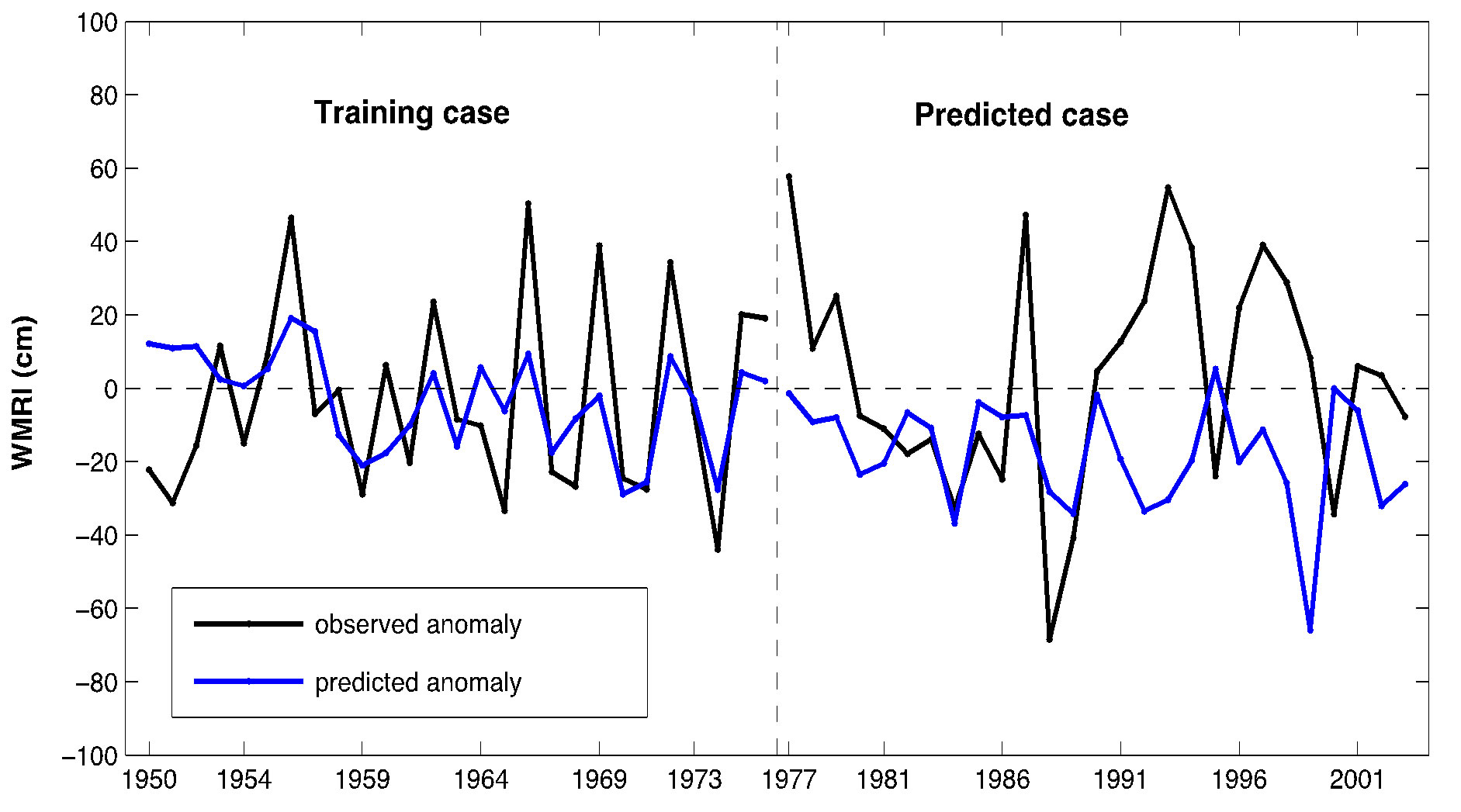 (c)
(c)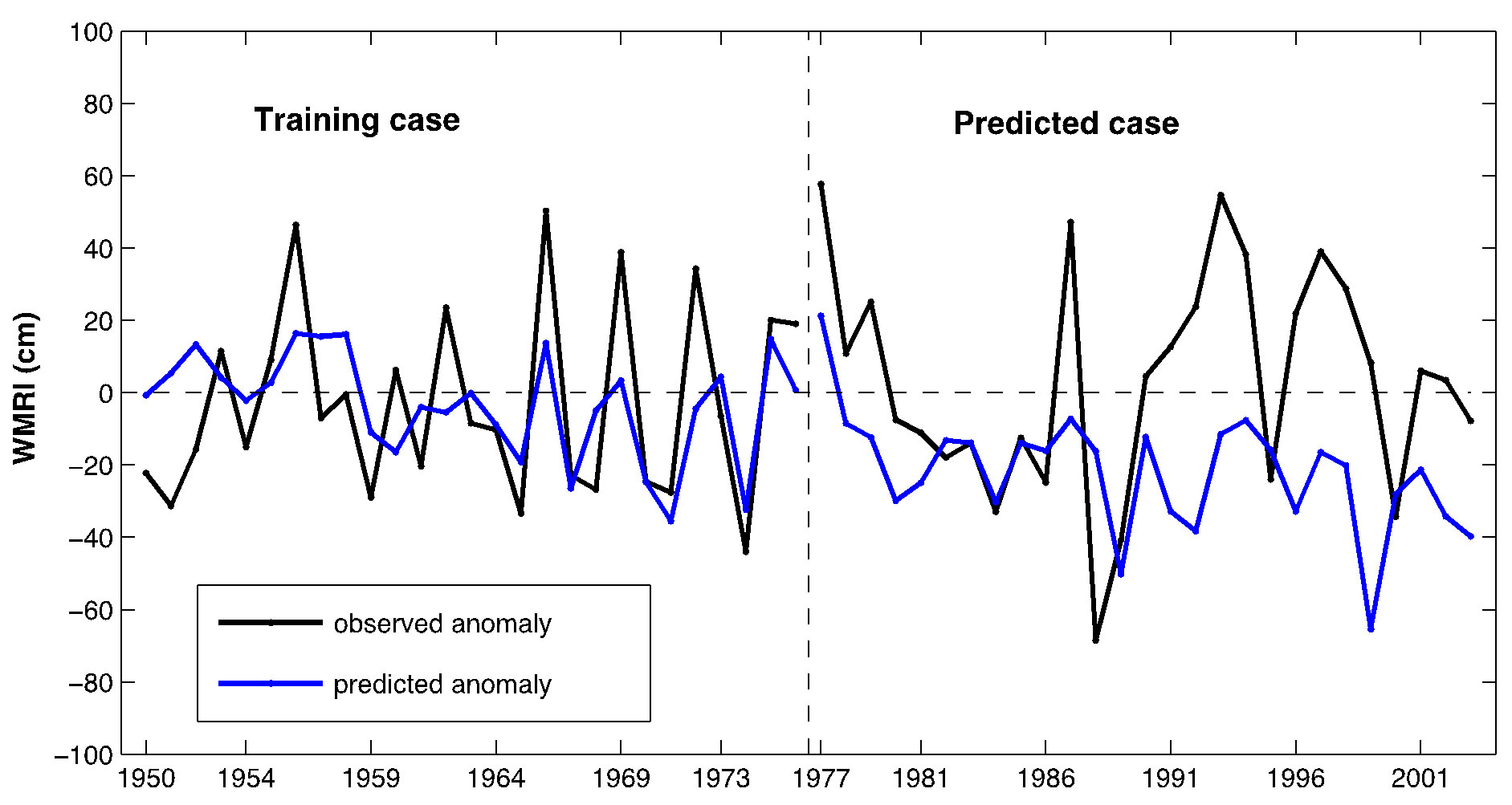 (d)
(d) (e)
(e)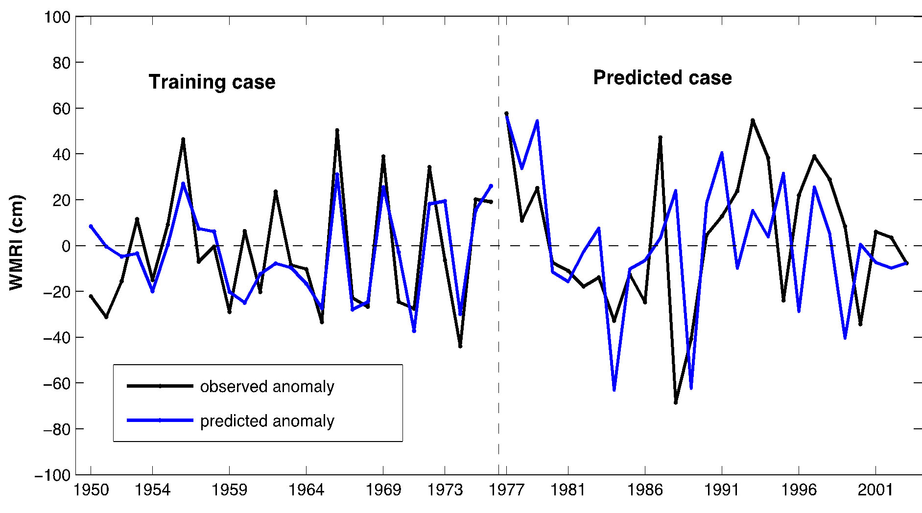 (f)
(f)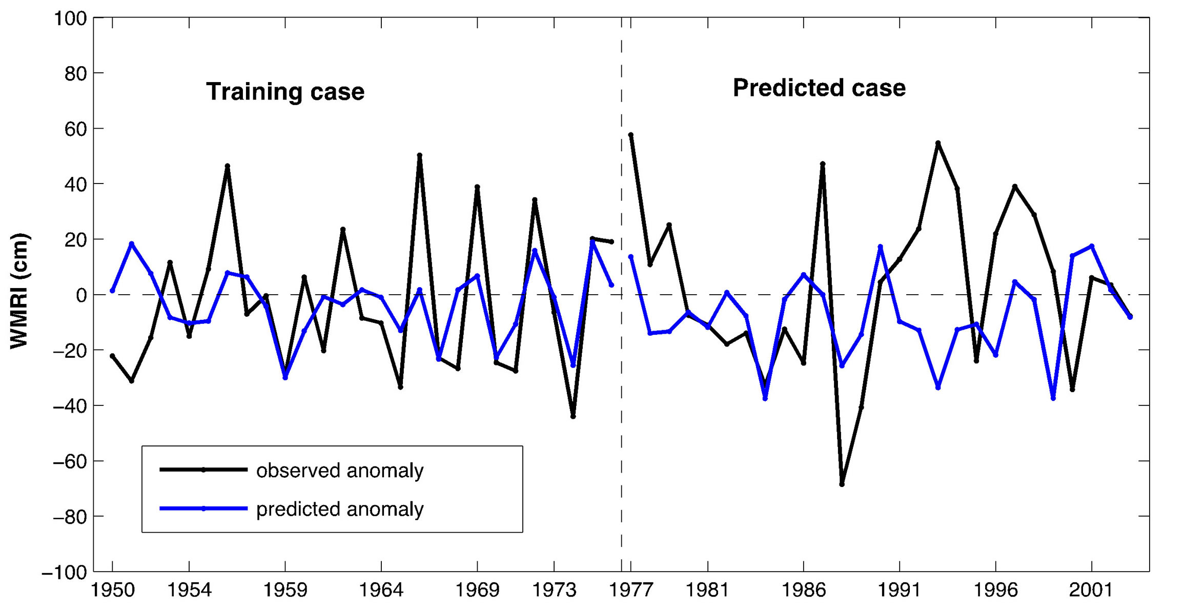 (g)
(g)
Figure 4. (a)-(g) Comparison of model output WMRI with observed WMRI in training and predicted case for (a) ACCI (A) regression model, (b) ACCI (B) regression model, (c) BOBI regression model, (d) NEI regression model, (e) A + B multiple regression model, (f) A + B + C + D multiple regression model, and (g) Nino 3.4t–7 regression model.

Table 1. Geographical extent of various SST Indices.

Table 2. Performance of linear and multiple regression model for training and predicted case.
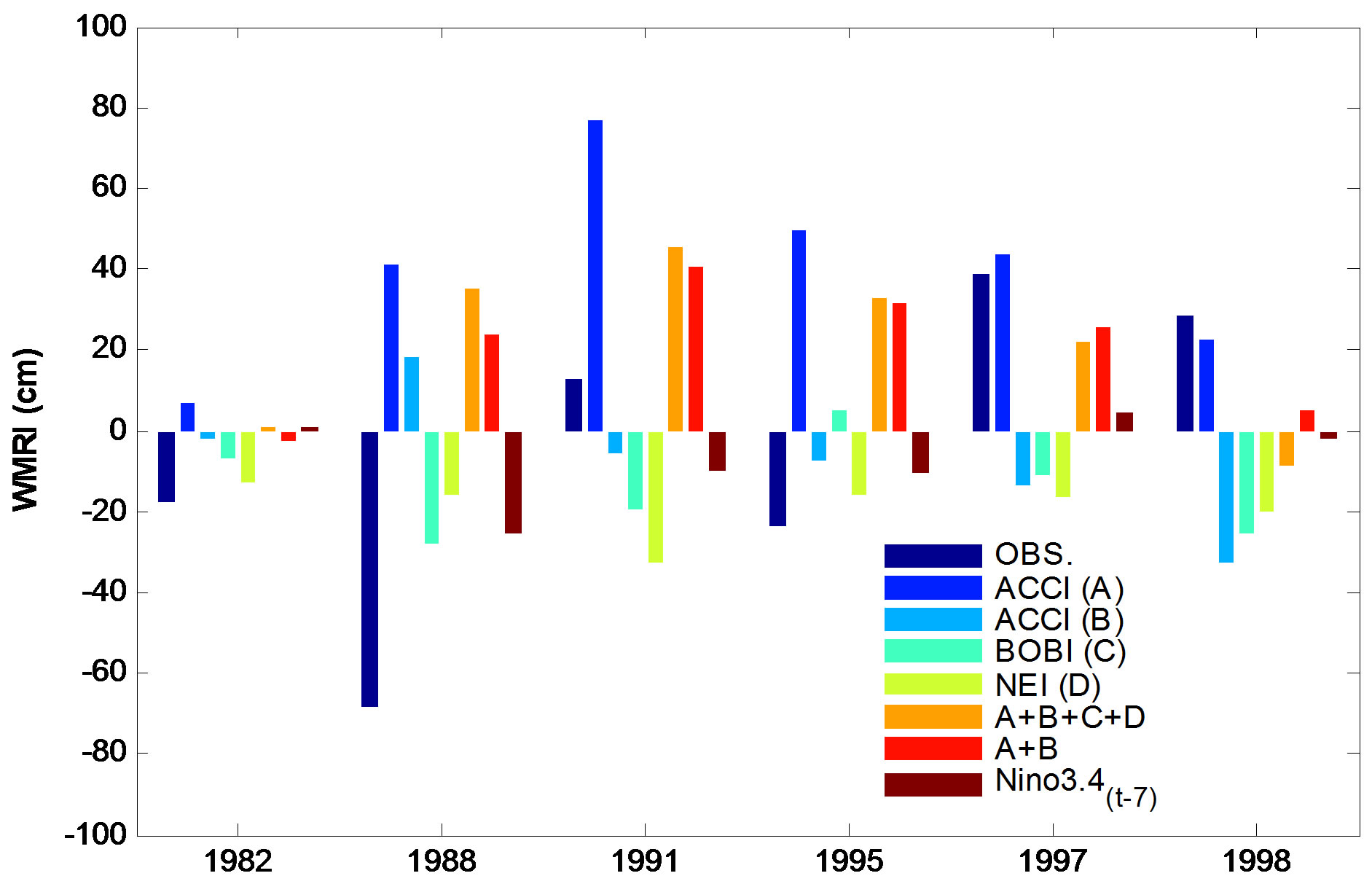
Figure 5. Comparison of model output WMRI with observed WMRI in predicted case for ENSO years (1982, 1988, 1991, 1995, 1997, 1998).
0.74 and 0.69 respectively in training case where as for predicated case the value are 0.51, 0.63, 0.56 and 0.51 respectively. It is clear that A + D multiple regression model is better with respect to all the models for the training and test cases both.
3.4. Categorical Forecast Skill Measures of Discrete Predictions
To evaluate the performance of the predictions of WMRI by linear and multiple regression models used in Sec. 3.2,

Table 3. The value of Willmott’s Index (WI) for various regression models in training and predicted case.
different categorical forecast skill scores measures are calculated. Normalised anomalies of predicted values of the Linear/Multiple regression models are calculated by subtracting arithmetic mean from the data and dividing with standard deviation of the dataset. Since the standard deviation of the normalized data is 1, a rare event happens when the modulus of the normalized observed precipitation exceeds 1. A normal event is one when the modulus of the normalized observed precipitation remains less than 1. A rare event is called “event” in this context. Following quantities are defined:
hit—event forecast to occur, and did occur miss—event forecast not to occur, but did occur false alarm—event forecast to occur, but did not occur correct negative—event forecast not to occur, and did not occur Some of the statistical skill score coefficients are calculated based on the above derived variables for validation of predictions. We have calculated accuracy, bias, Probability of Detection (POD), Probability of False Detection (POFD) and Threat Score (TS) [35].
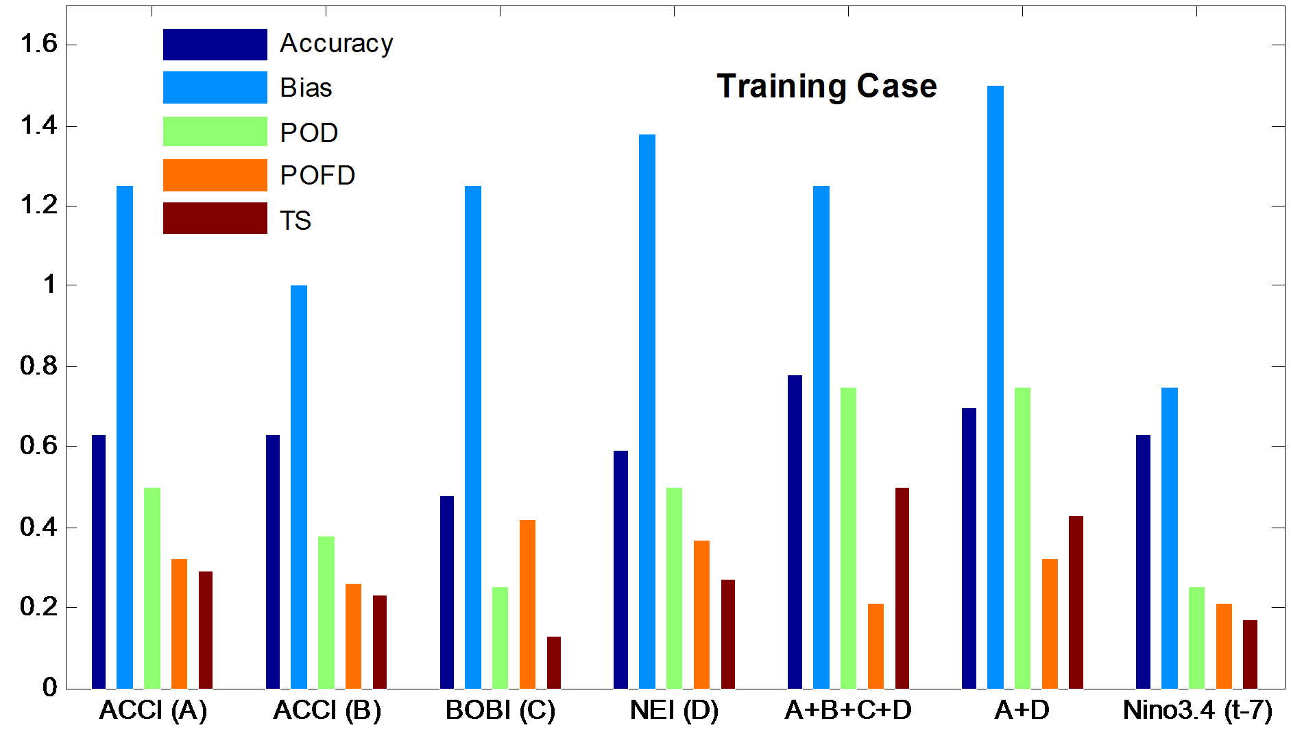
For training case (Figure 6(a)), accuracy is greater than 0.55 for most of regression models but it is 0.78 for A + B + C + D. Since the bias is greater than 1 in most of the cases except ACCIB (B) and Nino 3.4t–7, it can be argued that models are over predicting. Probability of detection (POD) is better (0.75) for A + B + C + D and A + D, indicating that both models are better in predicting rare event. Probability of false detection (POFD) is very small (0.21) for A + B + C + D multiple regression model which indicates that the fraction of “events” which were “wrongly” forecast is small. Threat Score (TS) measures accuracy when the correct negatives have removed from the forecast and it is found to be 0.50 and 0.43 for A + B + C + D multiple regression model and A + D multiple regression model, it strengthens our argument that the A + B + C + D multiple regression model and A + D multiple regression model is better than others.
For Predicted case (Figure 6(b)), it is interesting to mention that ACCI (A) and NEI (D) show same dichotomous skill scores for WMRI. Further A + B + C + D multiple regression model and A + D multiple regression model show same dichotomous skill scores. Since the dichotomous forecast skills refer to the capability of predicting the rare events only, we conclude that some members are equivalent when predicting the rare events.
In predicted case, Accuracy is greater than 0.55 for most of regression models except ACCI (B). Since the bias is less than 1 in most of the cases, it can be argued that models are under predicting except A + D multiple regression model, its value is 1. Probability of detection (POD) is better (0.33) for BOBI (C), A + D and Ninot–7. Probability of false detection (POFD) is very small (0.17) for ACCI (A) and Ninot–7 which indicates that the fraction of “events” which were “wrongly” forecast is small. Threat Score (TS) is found to be 0.25 and 0.20 for Ninot–7 and A + D models and it is 0.17 for ACCI (A). In prediction case, ACCI (A), A + D and Ninot–7 is better than the other models.
Thus, winter monsoon rainfall over South India predicted by linear and multiple linear regression models are comparable when El-Nino and La-Nina years are concerned. However, the overall prediction skill of the A + D multiple regression model is better than the other model.
 (a)
(a)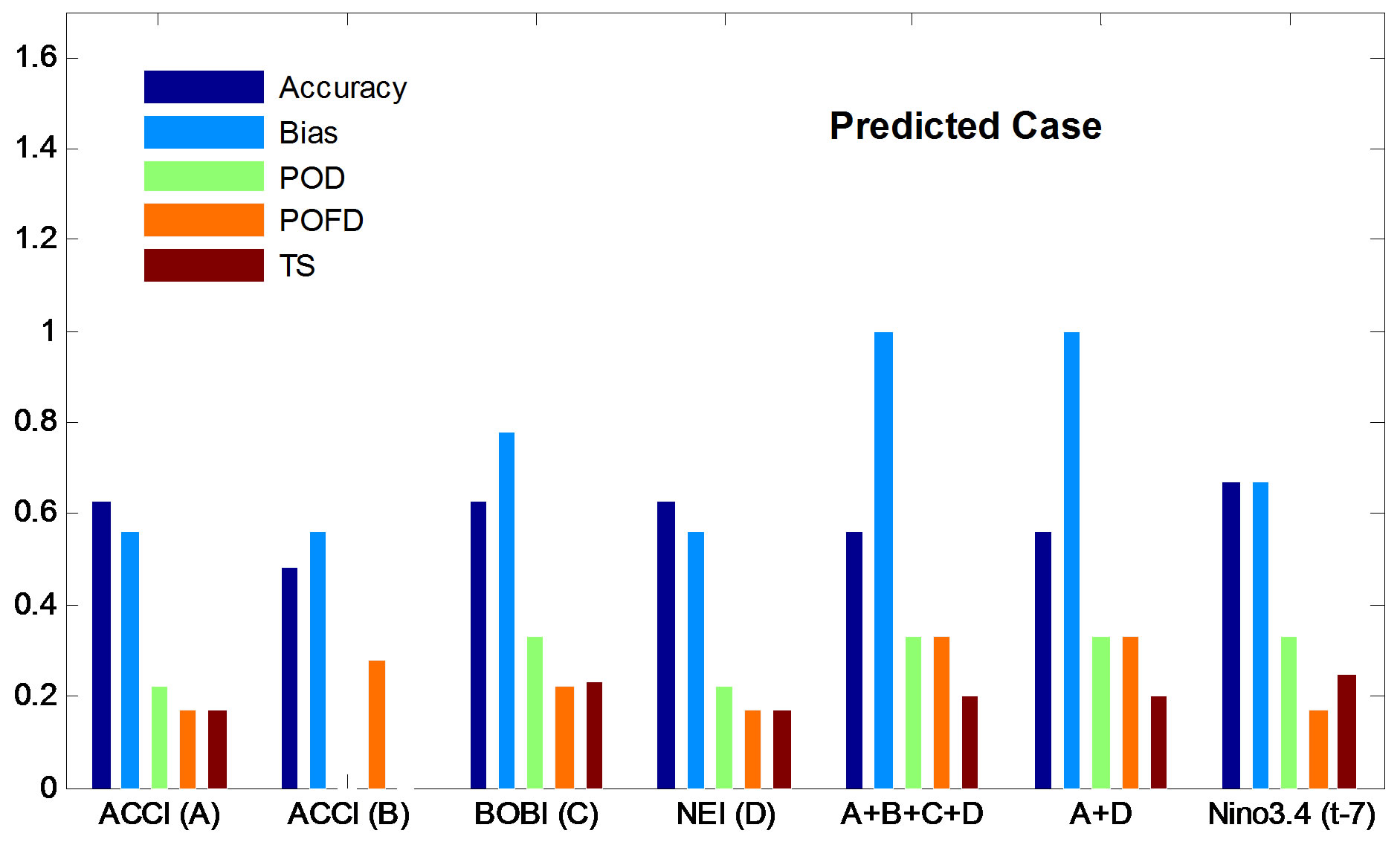 (b)
(b)
Figure 6. (a) (b) Prediction skill scores for training case and predicted case.
4. Conclusions
It is an established fact that SST anomalies in the STIO acts as predominant forcing of the Summer/Winter India Rainfall Index variability. In the present study, we have attempted to improve the seasonal forecast skill of the WMRI over South India. Correlation analysis between STIO with WMRI for the time period 1950-1976 reveals that there is significant lag correlation between them. Significant positive/negative correlations, with confidence level above 99% are found between WMRI and 1) ACCIA (A) with a lag of 1 season 2) ACCIB (B) with a lag of 5 seasons 3) BOBI with lag of 6 seasons (IV) NEI with lag of 7 seasons before the onset of winter monsoon. Correlation analysis is also done to see the effect of SST indices of Niño-3.4 regions on WMRI with a lag period of 1 - 8 seasons. Significant correlations, with confidence level above 99%, are found between WMRI and Niño- 3.4 index with a lag of 7 seasons before onset of winter monsoon. These SST indices are used for prediction of WMRI using linear/multiple linear regression models. Analysis of the predictive skill measures e.g. SD, RMSE, correlation coefficient and WI of the regression model reveals that the A + D regression model, is better as compared to other models. ACCIA and NEI model also have reasonable skill. However, the prediction skills remain inferior to those of the mean prediction, as it is observed by comparing the RMSE and SD of the observed precipitation in predicted case. The A + D regression model captures same sign for 4 ENSO years (1982, 1991, 1997, 1998) among six ENSO years. Forecast verification with respect to observation has been performed by categorical forecast techniques by calculating different skill score measures. It is found that for training case, A + B + C + D and A + D regression models are better in predicting rare events than the other models. For Predication case, ACCI (A) regression model, A + D multiple regression model and Ninot–7 regression model have better skill score than the other models.
Since the prediction and predictability of winter monsoon is still in an early stage and the present study will provide a basis idea of connectivity of southern and tropical Indian Ocean on a time span of 2 years. It is very difficult to propose any physical mechanism based on correlation analysis. Some modeling experiment may be performed to identify the physical mechanism behind this connectivity. This will strengthen our argument and provide the improvement in the accurate prediction of winter monsoon rainfall. The predictors defined in the present study may also be used to real time prediction of winter monsoon rainfall in South India.
5. Acknowledgements
First Author was supported by the Center for OceanLand-Atmosphere Studies (COLA) under grants from the National Science Foundation (0830068 and 0947837), the National Oceanic and Atmospheric Administration (NA09OAR4310058), and the National Aeronautics and Space Administration (NNX09AI84G). The second and third authors thank National Center for Antarctic and Ocean Research (NCAOR) and Indian National Center for Ocean Information Services (INCOIS), MoES, Govt. of India, for financial support.
REFERENCES
- C.-P. Chang, Z. Wang, and H. Harry, “The Asian Winter Monsoon,” In: B. Wang, Ed., The Asian Monsoon, Springer, Berlin Heidelberg, 2006, pp. 89-127. http://dx.doi.org/10.1007/3-540-37722-0_3
- G. T. Walker, “Correlation in Seasonal Variations of Weather, VIII. A Preliminary Study of World Weather,” Memoirs of the India Meteorological Department, Vol. 24, No. 4, 1923, pp. 75-131.
- G. T. Walker, “Correlation in Seasonal Variations of Weather, IX. A Further Study of World Weather,” Memoirs of the India Meteorological Department, Vol. 24, No. 9, 1924, pp. 275-333.
- A. K. Banerjee, P. N. Sen and C. R. V. Raman, “On Foreshadowing Southwest Monsoon Rainfall over Indian with Mid Tropospheric Circulation Anomaly of April,” Indian Journal of Meteorology, Hydrology and Geophysics, Vol. 29, 1978, pp. 425-431.
- D. R. Sikka, “Some Aspects of the Large Scale Fluctuations of Summer Monsoon Rainfall over India in Relation to Fluctuations in the Planetary and Regional Scale Circulation Parameters.,” Proceedings of the Indian Academy of Science (Earth and Planet Science), Vol. 89, 1980, pp. 179-195.
- T. P. Barnett, “Interaction of the Monsoon and Pacific trade Wind System at Interannual Time Scales Part I: The Equatorial Zone,” Monthly Weather Review, Vol. 111, No. 4, 1983, pp. 756-773. http://dx.doi.org/10.1175/1520-0493(1983)111<0756:IOTMAP>2.0.CO;2
- J. Shukla and D. A. Paolina, “The Southern Oscillation and Long Range Forecasting of the Summer Monsoon Rainfall over India,” Monthly Weather Review, Vol. 111, No. 9, 1983, pp. 1830-1837. http://dx.doi.org/10.1175/1520-0493(1983)111<1830:TSOALR>2.0.CO;2
- E. M. Rasmusson and T. H. Carpenter, “The Relationship between Eastern Equatorial Pacific Sea Surface Temperature and Rainfall over India and Sri Lanka,” Monthly Weather Review, Vol. 111, No. 3, 1983, pp. 517-528. http://dx.doi.org/10.1175/1520-0493(1983)111<0517:TRBEEP>2.0.CO;2
- D. A. Mooley and B. Parthasarathy, “Indian Summer monsoon and El Niño,” Pure and Applied Geophysics, Vol. 121, No. 2, 1984, pp. 339-352. http://dx.doi.org/10.1007/BF02590143
- B. Parthasarathy and G. B. Panth, “Seasonal Relationship between Indian Summer Rainfall and the Southern the Southern Oscillation,” Journal of Climate, Vol. 5, No. 4, 1985, pp. 369-378. http://dx.doi.org/10.1002/joc.3370050404
- J. Shukla and D. A. Mooley, “Empirical Prediction of the Summer Monsoon Rainfall over India,” Monthly Weather Review, Vol. 115, No. 3, 1987, pp. 695-703. http://dx.doi.org/10.1175/1520-0493(1987)115<0695:EPOTSM>2.0.CO;2
- P. J. Webster and S. Yang, “Monsoon and ENSO: Selectively Interactive Systems,” Quarterly Journal of the Royal Meteorological Society, Vol. 118, No. 507, 1992, pp. 877-926. http://dx.doi.org/10.1002/qj.49711850705
- J. Ju and J. M. Slingo, “The Asian Summer Monsoon and ENSO,” Quarterly Journal of the Royal Meteorological Society, Vol. 121, No. 525, 1995, pp. 1133-1168. http://dx.doi.org/10.1002/qj.49712152509
- B. P. Kirtman and J. Shukla, “Influence of the Indian Summer Monsoon on ENSO,” Quarterly Journal of the Royal Meteorological Society, Vol. 126, No. 562, 1997, pp. 213-239. http://dx.doi.org/10.1002/qj.49712656211
- K. Krishna Kumar, B. Rajagopalan and M. Cane, “On the Weakening Relationship between the Indian Monsoon and ENSO,” Science, Vol. 284, No. 5423, 1999, pp. 2156-2159. http://dx.doi.org/10.1126/science.284.5423.2156
- V. Krishnamurthy, and B. N. Goswami, “Indian MonsoonENSO Relationship on Interdecadal Timescale,” Journal of Climate, Vol. 13, No. 3, 2000, pp. 579-595. http://dx.doi.org/10.1175/1520-0442(2000)013<0579:IMEROI>2.0.CO;2
- V. Thapliyal, “Stochastic Dynamic Model for Long Range Forecasting of Summer Monsoon Rainfall in Peninsular India,” Mausam, Vol. 33, 1982, pp. 399-404.
- K. K. Krishna, M. K. Soman and K. K. Rupa, “Seasonal Forecasting of Indian Summer Monsoon Rainfall: A Review,” Weather, Vol. 50, 1995, pp. 449-467.
- M. Rajeevan, P. Guhathakurta and V. Thapliyal, “New Models for Long Range Forecasts of Summer Monsoon Rainfall over Northwest and Peninsular India,” Meteorology and Atmospheric Physics, Vol. 73, 2000 pp. 211- 225. http://dx.doi.org/10.1007/s007030050074
- T. DelSole and J. Shukla, “Linear Prediction of Indian Monsoon Rainfall,” Journal of Climate, Vol. 15, No. 24, 2002, pp. 3645-3658. http://dx.doi.org/10.1175/1520-0442(2002)015<3645:LPOIMR>2.0.CO;2
- R. P. Shukla, K. C. Tripathi, A. C. Pandey and I. M. L. Das, “Prediction of Indian Summer Monsoon Rainfall Using Nino Indices: A Neural Network Approach,” Atmospheric Research, Vol. 102, No. 1-2, 2011, pp. 99-109. http://dx.doi.org/10.1016/j.atmosres.2011.06.013
- K. V. Rao, “A Study of the Indian Northeast Monsoon Season,” Indian Journal of Meteorology, Hydrology and Geophysics, Vol. 14, 1963, pp. 143-155.
- A. Krishanan, “An Analysis of Trends in the Rainfall and Droughts Occurring in the Southwest and Northeast Monsoon Systems in the South Peninsular Indian,” Mausam, Vol. 35, 1984, pp. 379-386.
- O. N. Dhar, P. R. Rakhecha and A. K. Kulkarni, “Fluctuations in Northeast Monsoon Rainfall of Tamil Nadu,” Journal of Climatology, Vol. 2, No. 4, 1982, pp. 339-345. http://dx.doi.org/10.1002/joc.3370020404
- N. Singh and N. A. Sontakke, “On the Variability and Prediction of Rainfall in the Post Monsoon Season over India,” International Journal of Climatology, Vol. 19, 1999, pp. 309-339. http://dx.doi.org/10.1002/(SICI)1097-0088(19990315)19:3<309::AID-JOC361>3.0.CO;2-#
- G. Nageswara Rao, “Variations of the SO Relationship with Summer and Winter Monsoon Rainfall over India: 1872-1993,” Journal of Climatology, Vol. 5, 1999, pp. 3486-3495.
- P. Kumar, K. R. Kumar, M. Rajeevan and A. A. Munot, “Interannual Variability of Northeast Monsoon Rainfall over South Peninsular India: Teleconnections and Long Range Forecasting,” Conference on Monsoon Environments: Agricultural and Hydrological Impacts of Seasonal variability and Climate Change, ICTP, Trieste, 24-28 March 2003.
- J. Shukla and M. J. Fennessy, “Simulation and Predictability of Monsoons,” Proceedings of International Conference on Monsoon Variability and Prediction Technical Report WCRP-84, Geneva, World Climate Research Programme, 1994, pp. 567-575.
- O. S. R. U. Bhanu Kumar, C. V. Naidu and S. R. L. Rao, “Influence of the ENSO and the IOD on Indian Winter Monsoon Rainfall,” 14th Global Warming Conference, Bostan, 27-31 May 2003.
- R. H. Kripalani and P. Kumar, “Northeast Monsoon Rainfall Variability over South Peninsular India Vis-à-Vis the Indian Ocean Dipole Mode,” International Journal of Climatology, Vol. 24, No. 10, 2004, pp. 1267-1282. http://dx.doi.org/10.1002/joc.1071
- O. S. R. U. Bhanu Kumar, C. V. Naidu and S. R. L. Rao, “Prediction of Southern Indian Winter Monsoon Rainfall from September Local Upper-Air Temperatures,” Meteorological Applications, Vol. 11, No. 3, 2004, pp. 189- 199. http://dx.doi.org/10.1017/S1350482704001306
- T. M. Smith and R. W. Reynolds, “Improved Extended Reconstruction of SST (1854-1997),” Journal of Climate, Vol. 17, No. 12, 2004, pp. 2466-2477. http://dx.doi.org/10.1175/1520-0442(2004)017<2466:IEROS>2.0.CO;2
- K. E. Trenberth, “The Definition of El Nino,” Bulletin of the American Meteorological Society, Vol. 78, No. 12, 1997, pp. 2771-2777. http://dx.doi.org/10.1175/1520-0477(1997)078<2771:TDOENO>2.0.CO;2
- K. E. Trenberth and D. P. Stepaniak, “Indices of El Niño Evolution,” Journal of Climate, Vol. 14, No. 8, 2001, pp. 1697-1701. http://dx.doi.org/10.1175/1520-0442(2001)014<1697:LIOENO>2.0.CO;2
- D. S. Wilks, “Statistical Methods in Atmospheric Sciences,” Academic Press, California, 1995. pp. 169-390.
- C. J. Wilmott, “Some Comments on the Evaluation of Model Performance,” Bulletin of the American Meteorological Society, Vol. 63, No. 11, 1982, pp. 1309-1313. http://dx.doi.org/10.1175/1520-0477(1982)063<1309:SCOTEO>2.0.CO;2
- A. C. Comrie, “Comparing Neural Networks and Regression Models for Ozone Forecasting,” Journal of the Air & Waste Management Association, Vol. 47, No. 6, 1997, pp. 653-663. http://dx.doi.org/10.1080/10473289.1997.10463925
- G. Ibarra-Berastegi, A. Elias, A. Barona, J. Sáenz, A. Ezcurra and J. Díaz de Argandofia, “From Diagnosis to Prognosis for Forecasting Air Pollution Using Neural Networks: Air Pollution Monitoring in Bilbao,” Environmental Modelling & Software, Vol. 23, 2008, pp. 622- 637.
- C. J. Wilmott, S. G. Ackleson, R. E. Davis, J. J. Feddema, K. M. Klink, D. R. Legates, J. O’Donnell and M. C. Rowe, “Statistics for the Evaluation and Comparison of Models,” Journal of Geophysical Research, Vol. 90, No. C5, 1985, pp. 8995-9005. http://dx.doi.org/10.1029/JC090iC05p08995
NOTES
*Corresponding author.