Journal of Signal and Information Processing
Vol.3 No.4(2012), Article ID:24958,19 pages DOI:10.4236/jsip.2012.34057
Model Reduction of 2-D IIR Filters
![]()
1Science and Technology Department, University of Djelfa, Djelfa, Algeria; 2National Institute for Research & Development in Informatics, Bucharest, Romania.
Email: l_mitiche@yahoo.fr, amelmitiche@yahoo.fr, kacem.omar@yahoo.fr, vsima@ici.ro
Received June 24th, 2012; revised September 11th, 2012; accepted September 23rd, 2012
Keywords: Stability; Recursively Computable; Linear Phase; State Space; Balanced Realization; Model Reduction
ABSTRACT
The work presented in this paper concerns with analysis and synthesis of the two-dimensional Infinite Impulse Response (IIR) filters based on model order reduction. The synthesis is performed with two methods, the Prony’s method (Prony modified) and Iterative method, in the spatial domain, and with the method of Semi-Definite iterative Programming (SDP), in the frequency domain. After synthesis, we make an order reduction of the filter model by the QuasiGramians method.
1. Introduction
The fields of two-dimensional digital signal processing and digital image processing have maintained tremendous vitality over the past four decades and there is a clear indication that this trend will continue. Advances in hardware technology provide capabilities in signal processing chips and microprocessors which were previously associated with mainframe computers. These advances allow sophisticated signal and image processing algorithms to be implemented in real time at a substantially reduced cost. New applications continue to be found and existing applications continue to expand in such diverse areas as communications, consumer electronics, medicine, defense, robotics, and geophysics.
At a conceptual level, there is a great deal of similarity between one-dimensional signal processing and twodimensional signal processing. In one-dimensional signal processing, the concepts discussed are filtering, Fourier transform, discrete Fourier transform, fast Fourier transform algorithms, and so on. In two-dimensional signal processing, we again are concerned with the same concepts.
At a more detailed level, however, considerable differences exist between one-dimensional and two-dimensional signal processing. For example, one major difference is the amount of data involved in typical applications. In speech processing, we have 10.000 data points to process in a second. However, in video processing, we would have 7.5 million data points to process per second. Another example is the absence of the fundamental theorem of algebra for two-dimensional polynomials.
One-dimensional polynomials can be factored as a product of lower-order polynomials. An important structure for realizing a one-dimensional digital filter is the cascade structure. In this case, the z-transform of the digital filter’s impulse response is factored as a product of lower-order polynomials and the realizations of these lower-order factors are cascaded. The z-transform of a two-dimensional digital filters impulse response cannot, in general, be factored as a product of lower-order polynomials and the cascade structure therefore is not a general structure for a two-dimensional digital filter realization [1]. Another consequence of the nonfactorability of a two-dimensional polynomial is the difficulty associated with issues related to system stability. In a one-dimensional system, the pole locations can be determined easily, and an unstable system can be stabilized without affecting the magnitude response by simple manipulation of pole locations. In a two-dimensional system, since poles are surfaces rather than points and there is no fundamental theorem of algebra, it is extremely difficult to determine the pole locations [2].
The paper presented here is related particularly to the synthesis of the two-dimensional infinite impulse response filters using model order reduction. There are two main parts of the paper. In the first part, the synthesis is done, both in the spatial domain, with two methods, the Prony’s method (modified Prony) and Iterative method, and in the frequency domain, with iterative SemiDefinite Programming (SDP). In the second part of this paper, we make an order reduction of the synthesized (designed) filter using the Quasi-Gramians approach.
2. Designing 2D-IIR Filters
An 2D-IIR filter with an arbitrary impulse response  cannot be realized since computing each output sample requires a too large number of arithmetic operations [1,2]. As a result, in addition to requiring
  to be real and stable, we require
  to have a rational z-transform corresponding to a recursively computable system.
2.1. The Design Problem
The problem of IIR filter design is to determine a rational and stable function  with a wedge support output mask that meets a given design specification. In other words, we wish to determine a stable computational procedure that is recursively computable and meets a design specification.
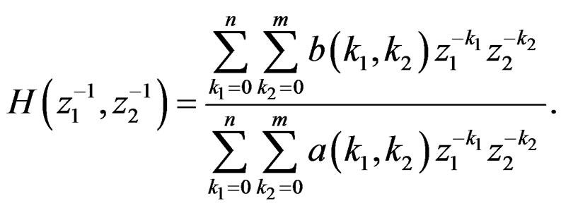
However, a given rational system function  can lead to many different computational procedures [1]. To make the relationship unique, we will adopt a convention in expressing
 . Specifically, we will assume that a(0, 0) is always 1, so
  will then be in the form
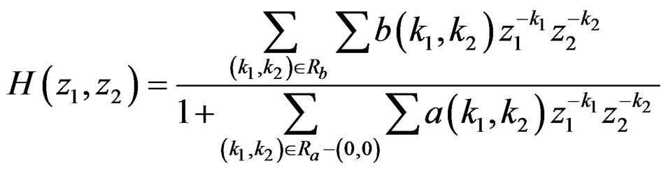 (1)
(1)
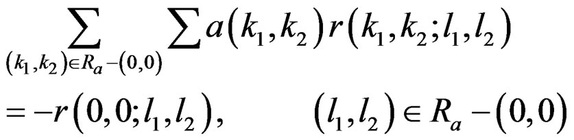
where Ra –(0, 0) represents the support region of  without the origin (0, 0), and Rb represents the support region of
 .
.
The unique computational procedure corresponding to (1) is then given by
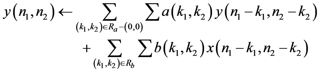 (2)
(2)
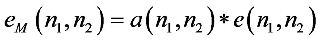
where the sequences  and
and  are the filter coefficients.
The first step in the IIR filter design is usually an initial determination of Ra and Rb, the support regions of  and
and . If we determine the filter coefficients by attempting to approximate some desired impulse response
  in the spatial domain, we will want to choose
  and
and  such that
  will have at least approximately the same support region as
 .
.
Another consideration is related to the filter specification parameters. In the low-pass filter design, for example, small ,
,  , (filter templates) and transition region will generally require a larger number of filter coefficients. It is often difficult to determine the number of filter coefficients required to meet a given filter specification for a particular design algorithm, and an iterative procedure may become necessary [1].
One major difference between IIR and FIR filters is related to stability. A FIR filter is always stable as long as  is bounded (finite) for all
 , so stability is never an issue. With an IIR filter, however, ensuring stability is a major task. One approach to designing a stable IIR filter is to impose a special structure on
  such that testing the stability and stabilizing an unstable filter become relatively easy tasks. Such an approach, however, tends to impose a severe constraint on the design algorithm or to highly restrict the class of filters that can be designed [1]. For example, if
  has a separable denominator polynomial of the form
 , testing the stability and stabilizing an unstable
  without affecting the magnitude response is a 1-D problem. However, the class of filters that can be designed with a separable denominator polynomial without a significant increase in the number of coefficients in the numerator polynomial of
  is restricted. An alternative approach is to design a filter without considering the stability issue, and then test the stability of the resulting filter and attempt to stabilize it if it proves unstable. However, testing stability and stabilizing an unstable filter are not easy problems.
In the 1-D case, there are two standard approaches to designing IIR filters. One is to design the filter from an analog system function. And the other is to design directly in the discrete domain. The first approach is typically much simpler and more useful than the second: using an elliptic analog filter’s system function and a bilinear transformation. Unfortunately, this approach is not useful in the 2-D case. In the 1-D case, this approach exploits the availability of many simple methods to design 1-D analog filters. Such simple methods do not exist for the design of 2-D analog filters. The second approach is the design of IIR filter directly in the discrete domain, can be classified into two categories. The first is the spatial domain design technique, where filters are designed by using an error criterion in the spatial domain. The second is the frequency domain design technique, where filters are designed by using an error criterion in the frequency domain. Therefore, the weighted Chebyshev error criterion, also known as the min-max error criterion, is a natural choice for designing IIR filters. An error criterion of this type, however, leads to a highly nonlinear problem [1,2].
2.2. The Stability Problem
In the 1-D case, testing the stability of a causal system whose system function is given by  is quite straightforward. Since a 1-D polynomial A(z) can always be factored straightforwardly as a product of first-order polynomials, we can easily determine the poles of H(z). The stability of the causal system is equivalent to having all the poles inside the unit circle. The above approach cannot be used in testing the stability of a 2-D first quadrant support system. That approach requires the specific location of all poles to be determined. Partly because a 2-D polynomial
  cannot in general be factored as a product of lower-order polynomials, it is extremely difficult to determine all the pole surfaces of
 , and the approach based on explicit determination of all pole surfaces has not led to successful practical procedures for testing the system stability [1,2].
2.3. Spatial Domain Design
The input often used in IIR filter design is , and the desired impulse response, assumed given, is denoted by
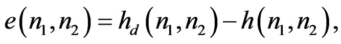
 . Spatial domain design can be viewed as a system identification problem. Suppose we have an unknown system that we wish to model with a rational system function
 . One approach to estimating the system model parameters (filter coefficients
  and
and  in our case), is to require the impulse response of the designed system to be as close as possible in some sense to
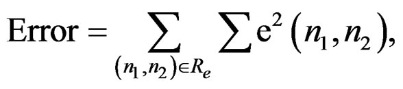
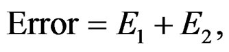
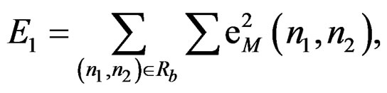
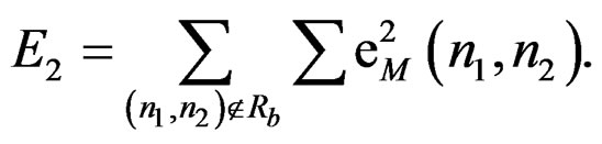
 . The error criterion used in the filter design is
 (3a)
(3a)
where
 (3b)
(3b)
and Re is the support region of the error sequence. Ideally, Re coincides with all values of . The mean square error in (3) is chosen because it is used widely in a number of system identification problems and some variation of it serves as the basis for a number of simple methods developed to estimate the system parameters.
Minimizing the error in (3) with respect to  and
and  is a nonlinear problem. An approach is to slightly modify the error in (3), so that the resulting algorithm leads to closed form solutions that require solving only sets of linear equations [1].
Consider a computational procedure given by
 (4)
(4)
We will assume that there are p unknown values of  and q + 1 unknown values of
 , and thus a total of N = p + q + 1 filter coefficients to be determined for a given pair
 .
.
Replacing  with
with  and
and  with
with  in (4) and noting that

is , we have
 (5)
(5)
Since we wish to approximate  as well as we can with
 , it is reasonable to define an error sequence
  as the difference between the lefthand and right-hand side expressions of (5)
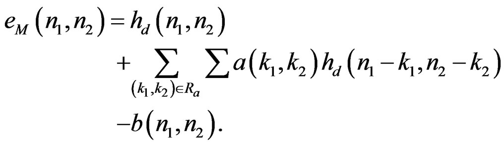 (6)
(6)
It is clear that  in (6) is not the same as
  in (3b). The subscript
  in
in  is used to emphasize that
  is a modification of
 . Minimizing
  with respect to the unknown coefficients
  and
and  is a linear problem.
a) Prony’s method
In Prony’s method, the error expression minimized is
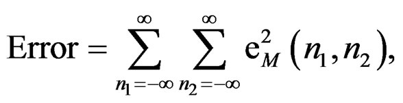 (7)
(7)
where  is given by (6).
The error in (7) is a quadratic form of the unknown parameters  and
and . Careful observation of the error in (7) shows that can be solved by first solving p linear equations for
  and then solving q + 1 linear equations for
 . It is useful to rewrite (7) as
 (8a)
(8a)
where
 (8b)
(8b)
and
 (8c)
(8c)
The expression  in (8b) consists of
  terms, and
  in (8c) consists of a large number of terms. Minimizing
  in (8) with respect to
  results in p linear equations for p unknowns given by
 (9a)
(9a)
where
 (9b)
(9b)
Once  is determined, we can minimize the error in (8a) with respect to
 .
.
Since Prony’s method attempts to reduce the total square error, the resulting filter is likely to be stable [2].
b) Iterative algorithm
The Iterative Algorithm is an extension of a 1-D system identification method developed by Steiglitz and McBride [1,2].
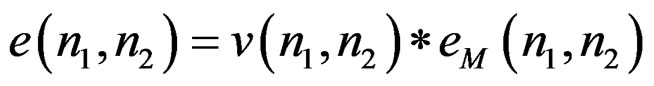
From (6), 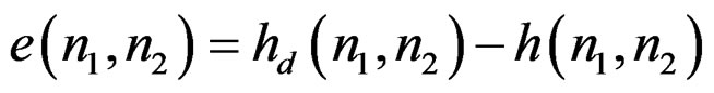 is related to
  by
by
 (10)
(10)
Equation (10) can be rewritten as
 (11)
(11)
The sequence  is the inverse of
 .
.
From (6) and (11)
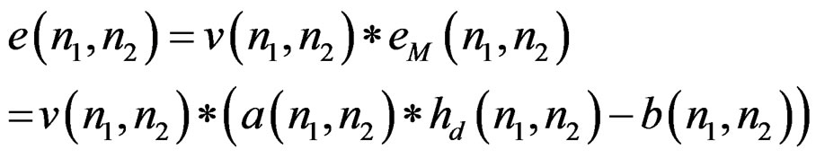 (12)
(12)
From (12), if  is somehow given, then
  is linear in both
  and
and , so minimization of
  with respect to
  and
and  is a linear problem.
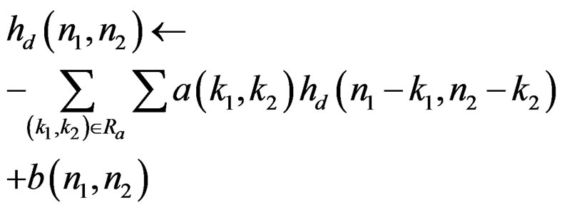
Algorithm
Step 1: We start with an initial estimate of , obtained following a method such as Prony.
Step 2: Obtain  from
from .
.
Step 3: Minimize  with respect to
  and
and  by solving a set of linear equations.
Step 4: We now have a new estimate of , and the process continues until we get a desired
  and
and .
.
c) Zero-phase filter design
One characteristic of a zero-phase filter is its tendency to preserve the shape of the signal component in the pass band region of the filter. In applications such as speech processing, the zero-phase (or linear phase) characteristic of a filter is not very critical. The human auditory system responds to short time spectral magnitude characteristics, so the shape of a speech waveform can sometimes change drastically without the human listener’s being able to distinguish it from the original. In image processing, the linear phase characteristic appears to be more important. Our visual world consists of lines, scratches, etc. A nonlinear phase distorts the proper registration of different frequency components that make up the lines and scratches. This distorts the signal shape in various ways, including blurring.
It is simple to design zero-phase FIR filters. It is impossible, however, for a single recursively computable IIR filter to have zero phase. To have zero phase,  must be equal to
 . An IIR filter requires an infinite extent
 , and output mask must have a wedge support. These requirements cannot all be satisfied at the same time. It is possible, however, to achieve zero-phase by using more than one IIR filter. A method particularly well suited to spatial domain design is to divide
  into different regions, design an IIR filter to approximate
  in each region, and then combine the filters by using a parallel structure.
Suppose we have a desired , we assume that
 (13)
(13)
We can divide  into an even number of regions: Two, four, six, eight, or more.
Suppose we divide  into four regions by
 (14a)
(14a)
 (14b)
(14b)
 (14c)
(14c)
and
 (14d)
(14d)
where  is a first-quadrant support sequence given by
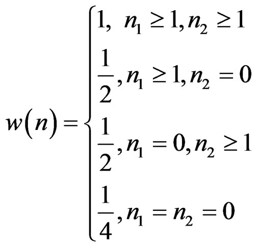 (15)
(15)
Suppose we use one of the spatial IIR filter design techniques discussed earlier to design  that approximates
 . Similarly, suppose we have designed
  that approximates
 . From (13) and (14),
 (16)
(16)
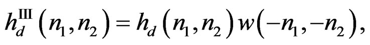
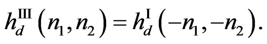
Therefore,  that approximates
  can be obtained from
  by
by
 (17)
(17)
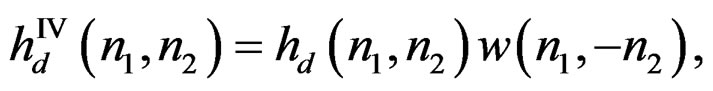
Similarly,  can be obtained from
  by
by
 (18)
(18)
Since ,
,  ,
,  , and
, and  approximate
 ,
,  ,
,  and
and , respectively,
  will be approximated by
  given by
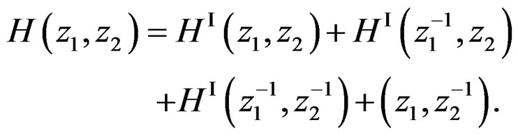
 (19)
(19)
 has zero phase since
  . The system in (19) can be implemented by using a parallel structure as shown in Figure 1. The input is filtered by each of the four recursively computable systems, and the results are combined to produce the output.
If  has fourfold symmetry,
 (20)
(20)
then  can be determined from
  by
by
 (21)
(21)
In this case,  in (19) is given by
 (22)
(22)
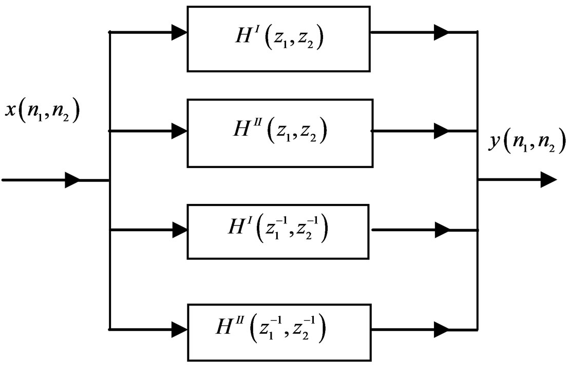
Figure 1. implementation of  using a parallel structure.
From (22), only one filter needs to be designed in this case.
2.4. Frequency Domain Design by the Iterative Semi-Definite Programming
Semi-definite programming (SDP) has recently attracted a great deal of research interest. Among other things, the optimization tool was proven to be applicable to the design of various types of FIR digital filters. An attempt on extending the SDP approach to 2-D IIR filters is made in [3]. Throughout this section the IIR filters are assumed to have separable denominators. This assumption simply imposes a constraint on the type of IIR filters being quadratically symmetric. Nevertheless, this class of filters is broad enough to cover practically all types of IIR filters that have been found useful in image/video [4].
Consider a quadratically symmetric 2-D IIR digital filter whose transfer function is given by
 , (23)
where
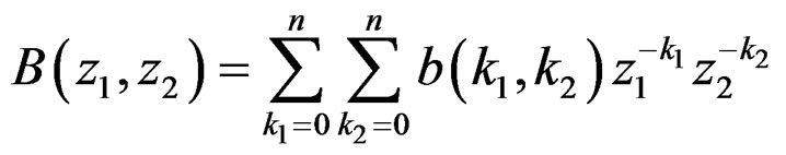
and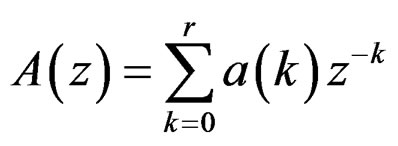 ,
, .
.
Since the filter is quadratically symmetric, we have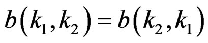 . As a result, there are only
  unknown variables in (23), which form a
  -dimension vector
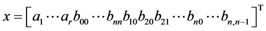 (24)
(24)
where . Denote the vector x in the kth iteration as
  and the frequency response of the filter for
  as
as . In the neighborhood of
 , the design variable can be expressed as
 .
.
The transfer function can be approximated in terms of a linear function of δ by
 (25)
(25)
where  is the gradient of de
  for
for .
.
Problem formulation
The min-max design is obtained as a solution of the following optimization problem:
Minimize  (26)
(26)
Subject to:
 (27)
(27)
with
 ,
,  , (28)
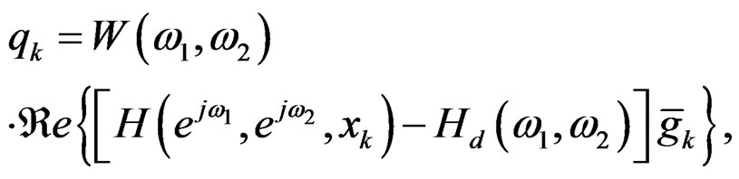
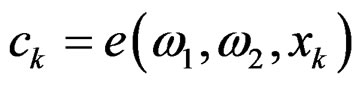
where μ is treated as an additional design variable, and
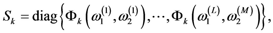 (29)
(29)
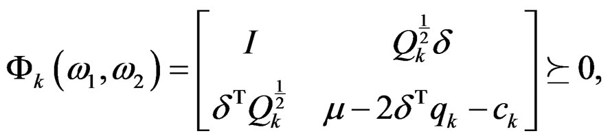 (30)
(30)
 (31)
(31)
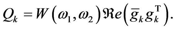
W(ω1, ω2) ≥ 0 is a weighting function,  the real part of (.), and
 (32)
(32)
 (33)
(33)
 is the desired frequency response, for
 where
where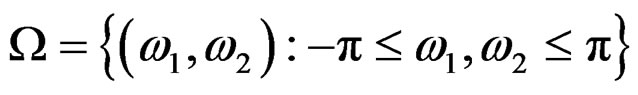 , and
, and
 (34)
(34)
where P is defined below and τ is a positive scalar that stability margin of the filter, and
 (35)
(35)
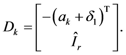
Denote the vectors formed from the first r components of  by
by . Since the denominator of
  is separable, it can be shown that the IIR filter with coefficient vector
  is stable if and only if the magnitudes of the eigenvalues of matrices
  are strictly less than one, where
  denote a matrix of size
  obtained by augmenting the identity matrix with a zero column on the right. Applying the wellknown Lyapunov theory [5], one concludes that matrix Dk is stable if and only if there exists a positive definite matrix P such that
 (36)
(36)
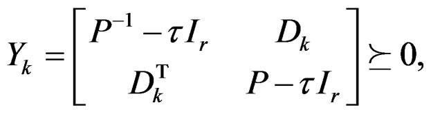
where  denotes that matrix M is positive definite. The matrix P in (34) is not considered as a design variable. Rather, this positive definite matrix is fixed in each iteration and can be obtained by solving the Lyapunov equation
 , (37)
where
 (38)
(38)
with P fixed in Yk, the minimization problem in (26) and (27) is an SDP problem of size 
Design steps
Given the order of the IIR filter (n, r) and the desired frequency response .
.
Step 1: The proposed design method starts with an initial point x0 that corresponds to a stable filter obtained using a conventional method.
Step 2: With this x0, a positive definite matrix P can be obtained by solving the Lyapunov equation (37), and the quantities Qk, qk, and ck can be evaluated by using (31)-(33).
Step 3: Next we solve the SDP problem in (26) and (27).
Step 4: The solution  obtained can be used to update x0 to x1 = x0 +
 . The iteration continues until
  is less than a prescribed tolerance ε.
3. Order Reduction
It is often desirable to represent a high order system by a lower order system. A suitable model reduction procedure should provide a model that approximates the original well, it should produce stable models from a stable original, and it should be able to be implemented on a computer with high computational efficiency and reduced memory requirements. The reduction of models in the state space (SS) realization environment has definite advantages. It is possible to apply the vast knowledge of matrix theory in the analysis, while the nonuniqueness of SS realization allows to choose of using one that is better suited for the purpose at hand [6,7].
3.1. State-Space Model
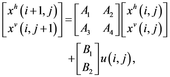
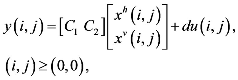
Roesser’s model is the following [6,7]:
 (39a)
(39a)
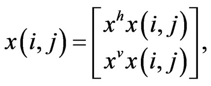
where x is the local state, xh, an n-vector, is the horizontal state, xv, an m-vector, is the vertical state, and
 (39b)
(39b)
 (39c)
(39c)
where u, the input, is an l-vector and y, the output, is a p-vector. Clearly xh, the horizontal state, is propagated horizontally, and xv, the vertical state is propagated vertically by first-order difference equations.
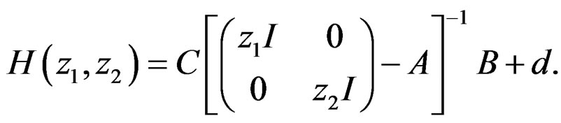
The 2-D transfer function can be written as:
 (40)
(40)
It is clear that there is a one-to-one correspondence between Roesser’s model and circuit implementations with delay elements  and
and .
.
3.2. Minimal State Space Realization
The minimal state-space realizations are not possible for all 2-D transfer functions [8]. However, minimal statespace realizations have been determined for a system with separable denominator [9].
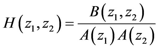
Consider the linear time-invariant 2-D system, described by the spatial transfer function [10]
 (41)
(41)
The numerator coefficients of (41) can be arbitrary, while the denominator coefficients satisfy the following relationship:
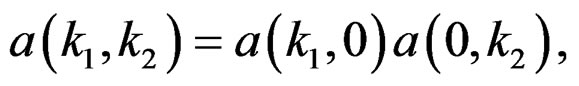 (42)
(42)
with 
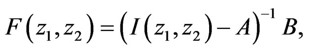
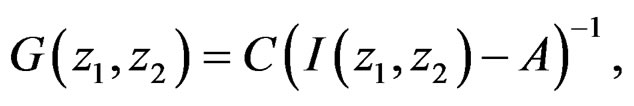
The state-space model sought is of the Givone-Roesser type [10], described with  and
and


 and C2 of dimension
 and
and  respectively.
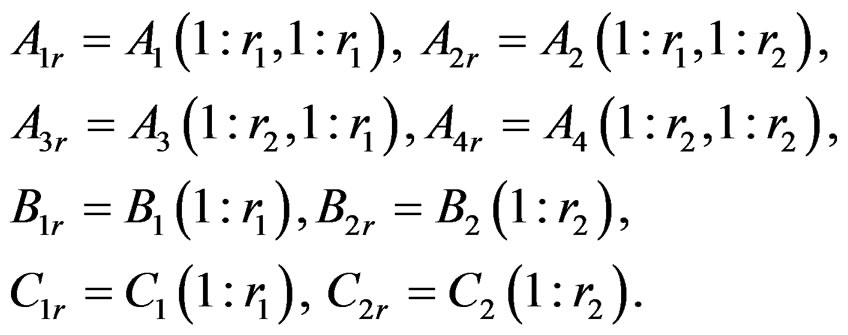
The minimal realization in this case requires only  dynamic elements. A realization of the statespace can be written as:
 ,
,
 ,
,
 where
where
and
 ,
,
 ,
, , and
, and  [11,12].
3.3. Model Order Reduction Methods
The most popular 1-D model reduction techniques are based on the concept of balanced realization which was originally proposed by Moore [13]. Given a discrete system, its balanced realization describes the system in a state-space representation in which the importance of the ith state variable can be measured by the ith Hankel singular value of the system. This suggest that one way of obtaining a low-order approximation of a state-space model is to form a balanced realization and then to retain those states corresponding to r largest Hankel singular values, where r is the order of the reduced-order system.
One of the problems in the study of 2-D model reduction is to extend the balanced realization concept to the 2-D case. Since a balanced realization is essentially determined by the controllability and observability Gramians of the system, and since there are several types of Gramians of the system that can be properly defined for a given 2-D system, there are different types of balanced realizations for a 2-D discrete system, leading to different balanced approximations [14].
3.3.1. Three Types of Gramians for 2-D Discrete Systems
Consider the Givone-Roesser state-space model of a SISO system described in (39), and define [14]
 (43a)
(43a)
 (43b)
(43b)
where 
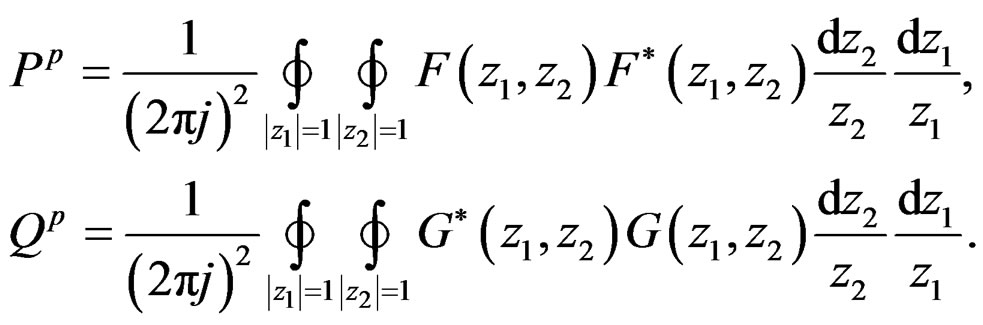
The first type of 2-D Gramians, known as the pseudocontrollability and observability Gramians [15], are defined as
The second type of Gramians, known as the structured controllability and observability Gramians [16], are defined by the positive definite solutions set of Ps and Qs Lyapunov inequalities
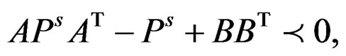
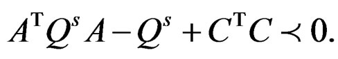
Note that the positive definite matrices Ps and Qs, if they exist, are not unique. This lead to the nonuniqueness of structurally balanced realizations that are based on Ps and Qs.
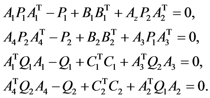
The third type of Gramians, known as quasi-controllability and observability Gramians [17], are defined by the positive definite block-diagonal matrices 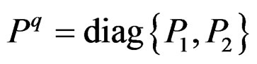 and
and 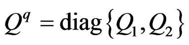 where Pi and Qi (i = 1,2) satisfy the Lyapunov equations:
In terms of computation complexity, the structured Gramians are the most expensive to evaluate while the quasi-Gramians are the most economical [14].
3.3.2. Balanced Realizations Approximation
Since there are at least three types of Gramians, one can accordingly derive three different types of balanced realizations. In effect, once a certain type of Gramians is chosen, the upper left and lower right diagonal blocks of the Gramians are used to compute the transformation matrix  by using, for example, Laub’s algorithm [18] such as the realization characterized by
  is balanced.
A reduced-order system of order , denoted by
  can be obtained by truncating the matrices A, B, and C as
 where [14]
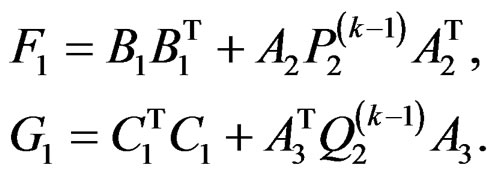
3.3.3. Iterative Algorithm for Computing the Quasi-Gramians
An iterative method for the computation of Quasi-Gramians is described, where each iteration involves solving two 1-D Lyapunov equations. For a 2-D stable system, the algorithm converges very quickly to the 2-D quasiGramians [19].
Step 1: Set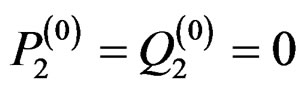 , and k =1.
Step 2: Solve the following 1-D Lyapunov equations for  and
and :
:
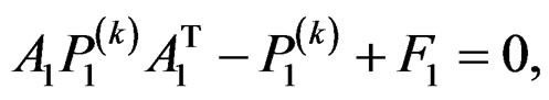 (44a)
(44a)
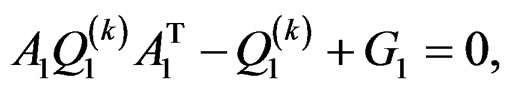 (44b)
(44b)
where
Step 3: Solve the following 1-D Lyapunov equations for  and
and :
:
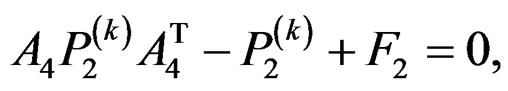 (44c)
(44c)
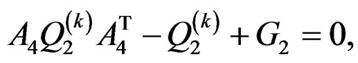 (44d)
(44d)
where
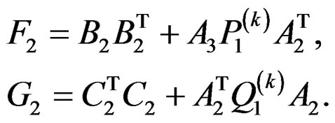
Step 4: Set k = k + 1 and repeat Steps 2 and 3 until
 ,
,
 .
.
where ε is a prescribed tolerance [19].
4. Illustrative Simulations
We have divided the simulation into two parts: 2D-filter design and order reduction. The interpretation of the results is given at the end of this section.
Part 1: 2D-filter design
The design has been performed in two domains (see Figures 2-7):
• Spatial domain by two methods: Prony’s method and the Iterative method.
The numerator  and the denominator
  matrices are generated, then we use the funcProny’s method
 (a)
(a)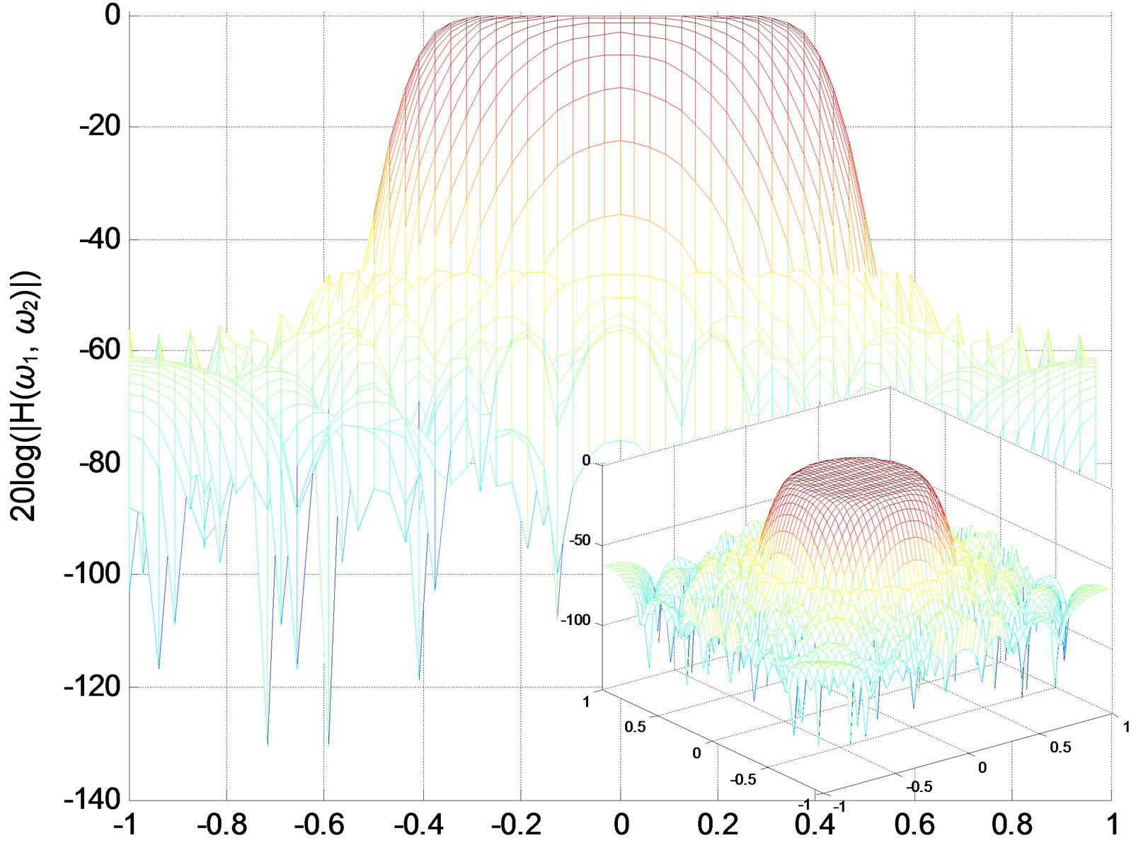 (b)
(b)
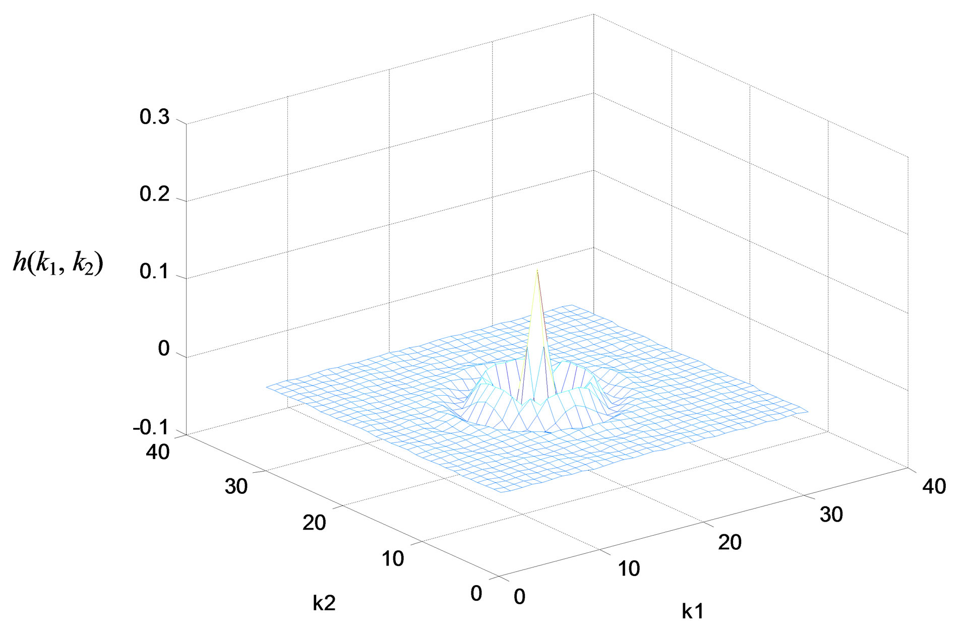
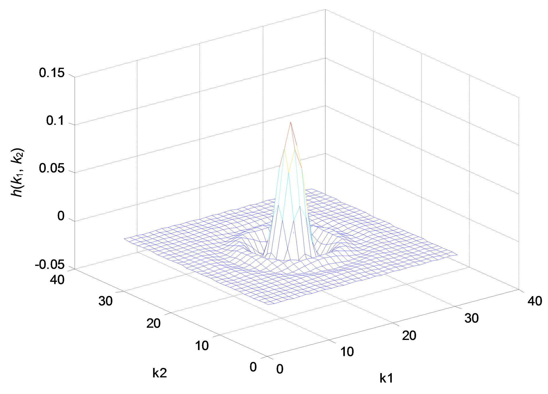
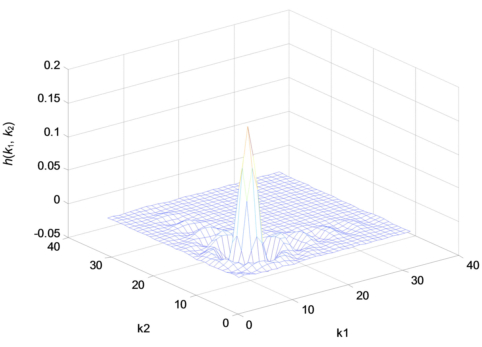
Figure 2. Zero-phase lowpass IIR filter. (a) Impulse response; (b) Amplitude responses (in decibels), “X-Z” perspective.
 (a)
(a)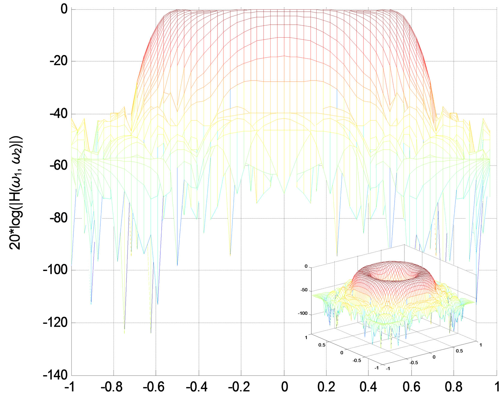 (b)
(b)
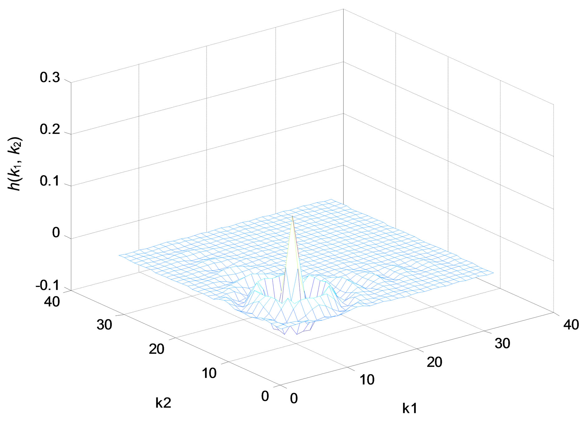
Figure 3. Zero-phase bandpass IIR filter. (a) Impulse response; (b) Amplitude responses (in decibels), “X-Z” perspective.
tion Impulse_2D.m to produce the impulse response and frequency response.
• Frequency domain, we use the method of Semidefinite Programming (SDP) to do the same.
For the Prony’s method and Iterative method the IIR digital filters are specified by the following templates:
Filter’s order 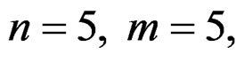 (the a and b matrix dimension).
The pass band and stop band corresponding to each type of filter are: Lowpass: Rp = [0 0.4], and Rs = [0.5 1].
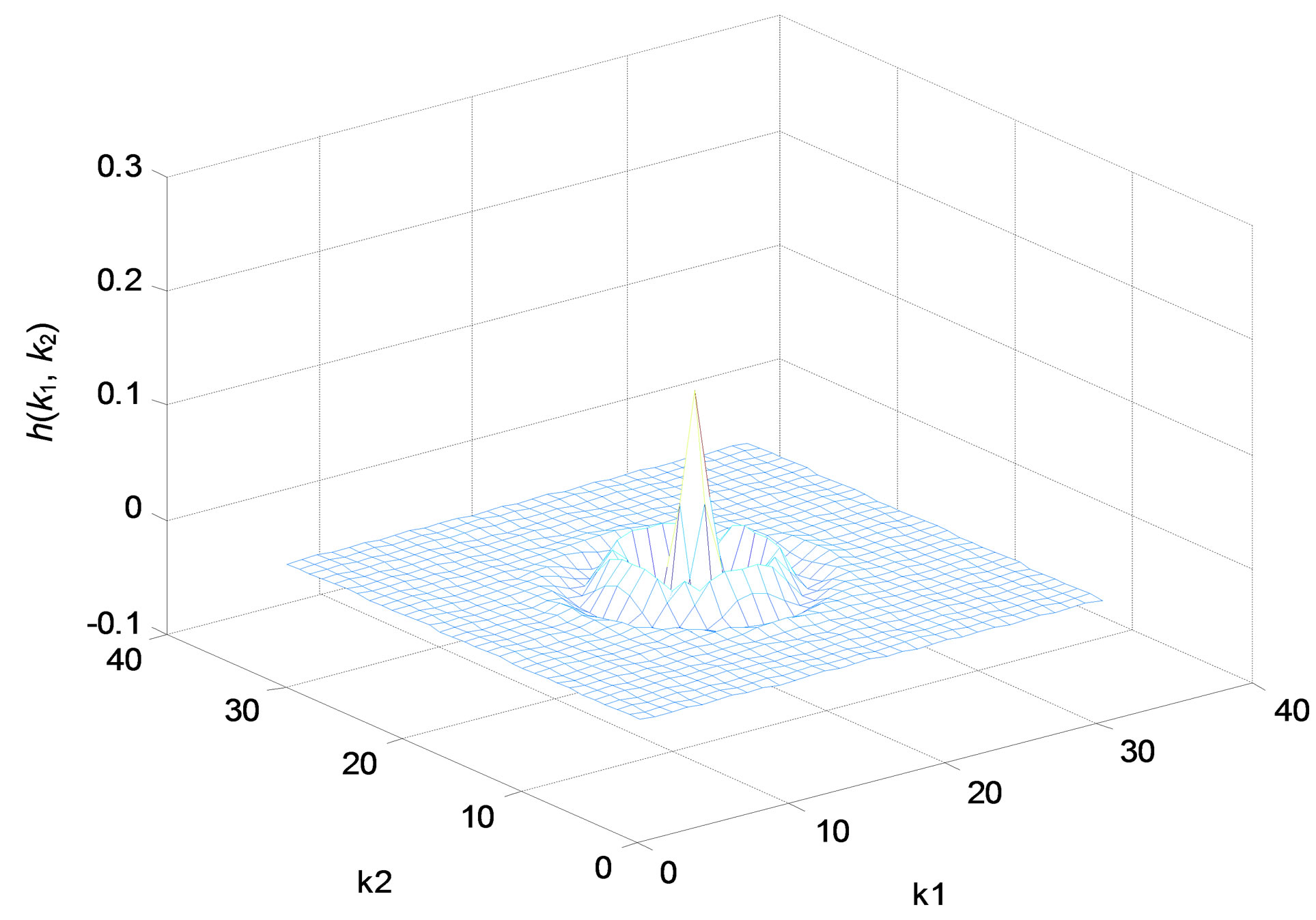
Iterative method
 (a)
(a)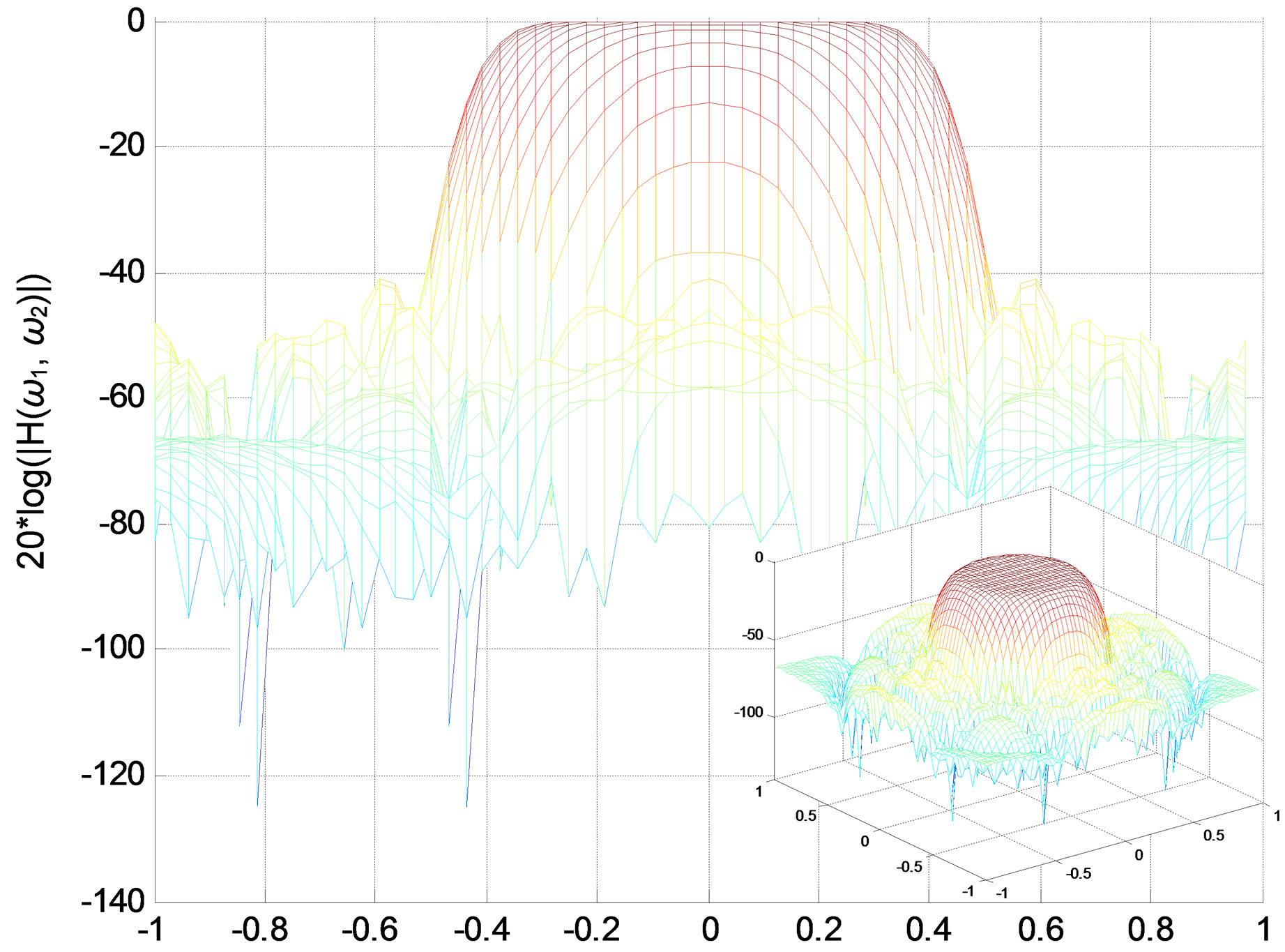 (b)
(b)
Figure 4. Zero-phase lowpass IIR filter. (a) Impulse response; (b) Amplitude responses (in decibels), “X-Z” perspective.
Bandpass: Rp = [0.4 0.6], Rs1 = [0 0.3] and Rs2 = [0.7 1].
For the SDP method, let IIR digital filters be specified by the following templates:
Filter order n = 13, m = 13 (the a and b matrix
 (a)
(a)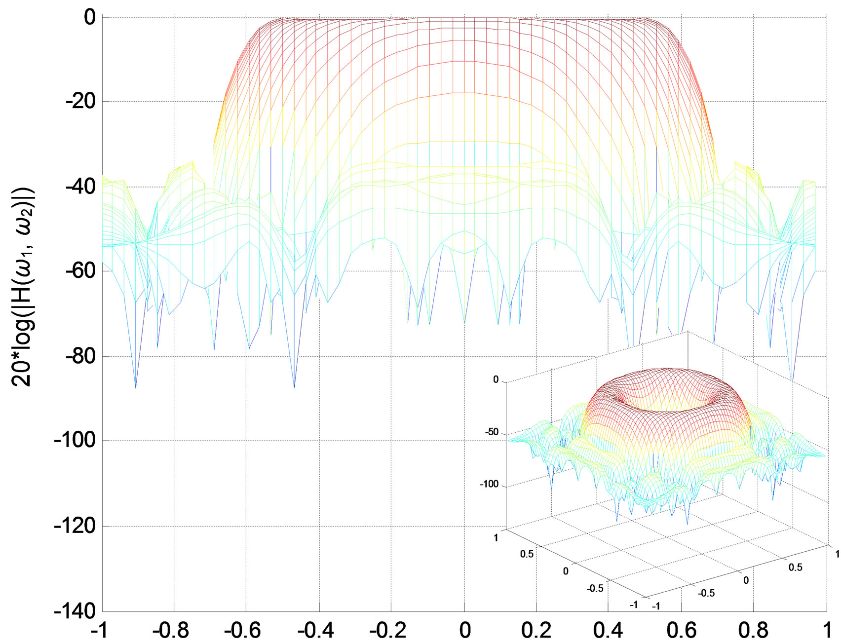 (b)
(b)
Figure 5. Zero-phase bandpass IIR filter. (a) Impulse response; (b) Amplitude responses (in decibels), “X-Z” perspective.
dimension).
The passband and stopband corresponding to each type of filter are:
Lowpass: Rp = [0 0.4], and Rs = [0.5 1].
Bandpass: Rp = [0.48 0.55], Rs1 = [0 0.3] and Rs2 = [0.7 1].
Number of iterations: it = 2.
Part 2: Order reduction
 (a)
(a)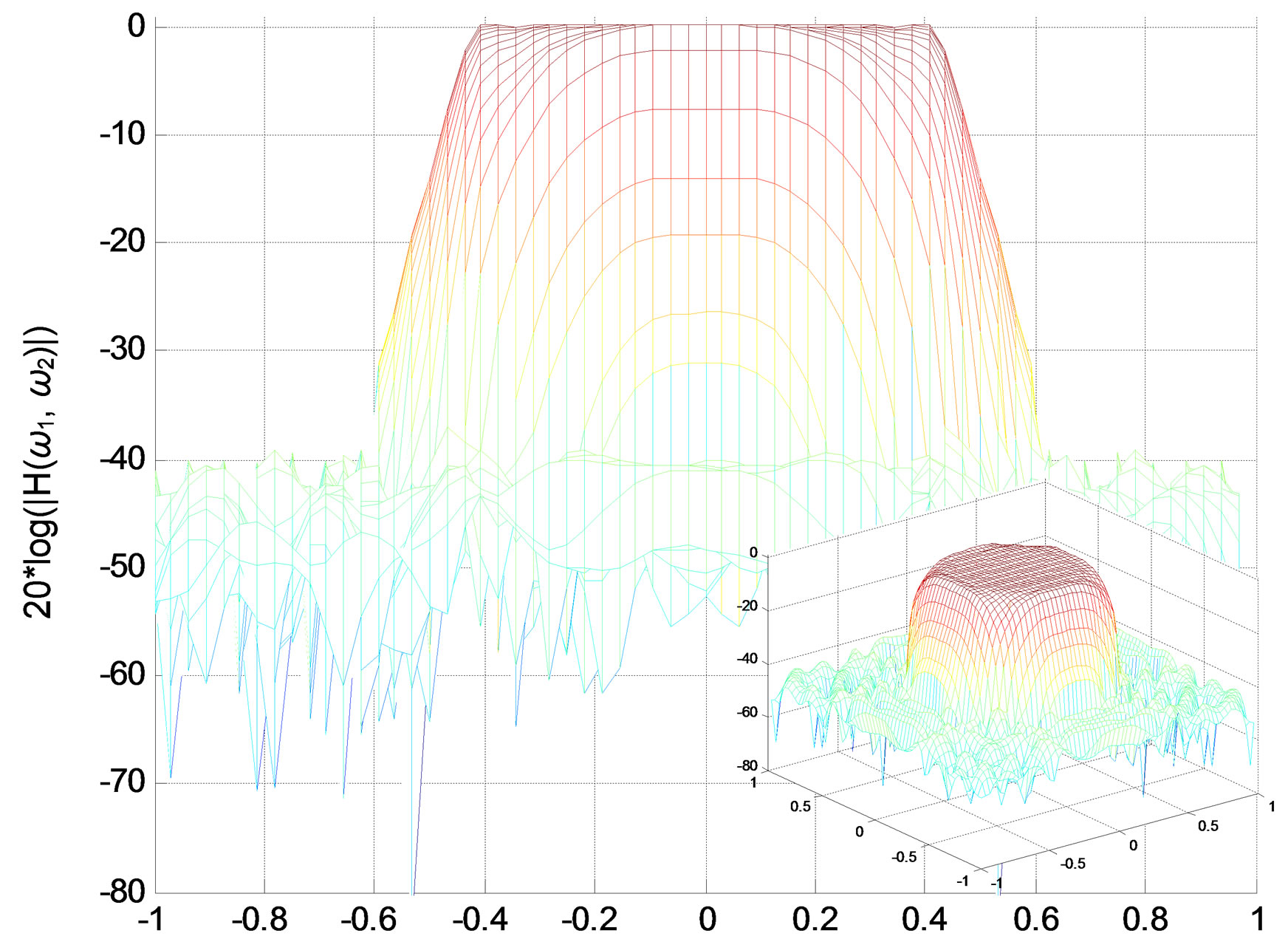 (b)
(b)
Figure 6. Lowpass IIR filter. (a) Impulse response; (b) Amplitude responses (in decibels), “X-Z” perspective.
We apply the method of Quasi-Gramians to the lowpass filter designed in the first part. First, we use our function tf2ss2_2D.m to transform the transfer function matrices a and b to the state-space model (A, B, C, d); then we applied the Quasi-Gramians method to produce a reduced-order model , (see Figures 8-11).
Iterative method
The order of original filter is: n = 5, m = 5; the total number of coefficient is:
 (a)
(a)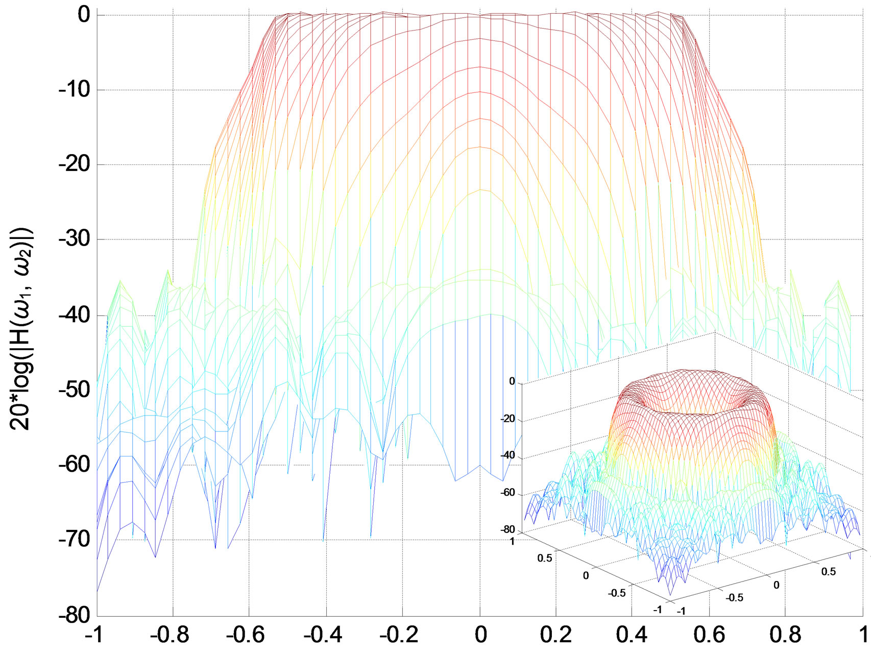 (b)
(b)
Figure 7. Bandpass IIR filter. (a) Impulse response; (b) Amplitude responses (in decibels), “X-Z” perspective.
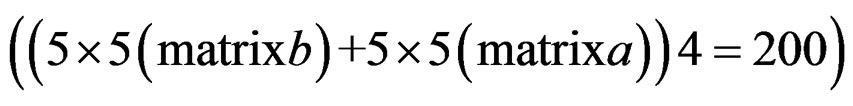 .
.
The dimensions of the matrices A, B, and C are ,
,  , and
, and , respectively.
Number of iterations is: it = 10.
Order of reduced filter is: r1 = 4, r2 = 5.
• The total number of coefficient is
 (a)
(a)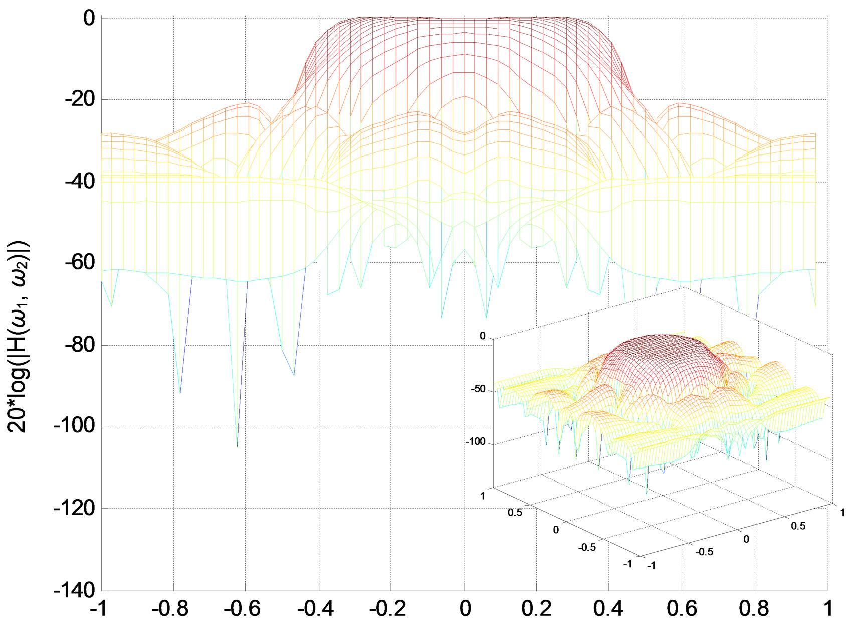 (b)
(b)
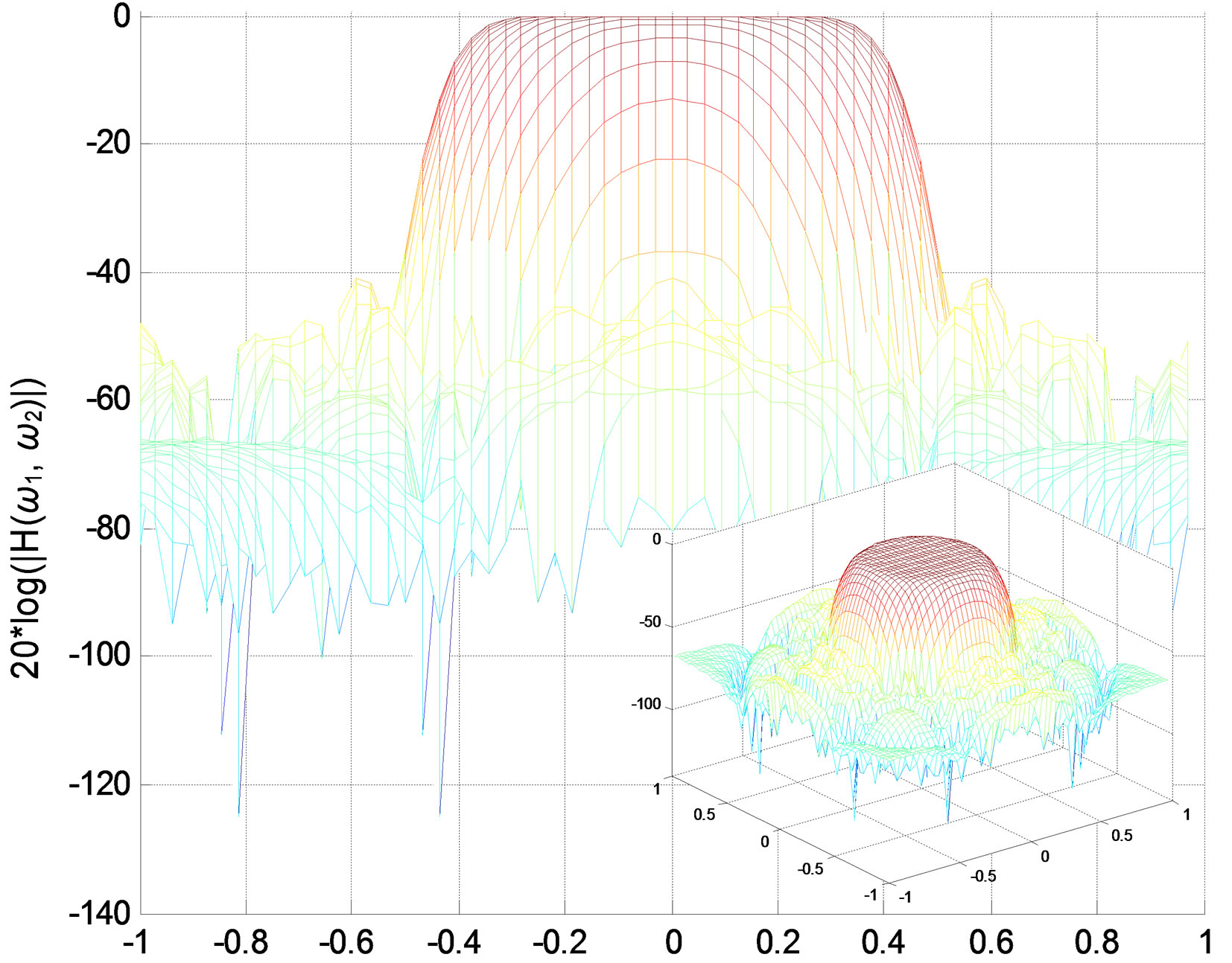
Figure 8. Lowpass IIR filter amplitude responses (in decibels), “X-Z” perspective. (a) Original filter 5 × 5 (200 coefficients); (b) Reduced-order filter 4 5, (160 coefficients).
 .
.
• Reduced-order filter  (160 coefficients).
SDP method
The order of original filter is: n =13, m = 13.
• The total number of coefficient is: .
.
• The dimensions of the matrices A, B, and C are 
 and
and respective-ly (minimal realization).
Number of iterations is: it = 2.
Order of reduced filter is: r1 = 8, r2 = 8.
• The total number of coefficient is: .
.
Interpretation
The results obtained lead to the following:
For the design, there is not much difference between the Prony method and the Iterative method. However, we can notice that there is a small improvement at stop-band (attenuation) when Iterative method is applied:
Prony:  (lowpass filter);
Iterative:  (lowpass filter).
And the results obtained with the SDP method are comparable to the other two methods, but we found a performance decrease in both bands (pass band and stopband). It is possible to improve the results by increasing number of coefficients (n, r) or the number of iterations. A good aspect of this method is the stability, which can be measured by the maximum of the roots of the column or row vectors of the denominator matrix “a”: we found the following results:
max (abs (roots (a (:, 1)))) = 0.8926 for the low-pass filter, and = 0.8578 for the bandpass filter.
where max, abs, and roots are Matlab functions [20].
*The order reduction:
• Since the filter designed by Prony and Iterative methods has a non-minimal realization, and the reduced filter can be unstable, the reduction results are not good (see Figures 8 and 9).
• But the stability is preserved in the SDP method:
For the original filter, max (abs (roots (a (:, 1)))) = 0.8926, and = 0.9119, for the reduced low-pass filter.
The results obtained show that the reduced low-pass filter is acceptable as the number of coefficients decreases from 338 to 128, and the max error between the reduced and original filter is max(E) ≤ 0.02 (cf. Figure 11).
5. Conclusions
In the design stage, stability and zero-phase of a 2-D IIR filter may become big problems. In 1-D we represent a pole or a zero by a point in a 2-D plan (real part and imaginary part), but in 2-D, the poles are surfaces in a 4-D plan, and so it is extremely difficult to test the stability and to stabilize an unstable filter. In image processing, the output image from a system (a filter in this case) can be deformed by the phase nonlinearity.
The reduction also suffers from some problems. The reduction in the state-space by conventional methods, for example, using a balanced transformation, requires a minimal realization of a transfer function in state-space, and then to find a method to compute the transformation matrix to a balanced model, which requires to maintain the stability and reduce as much as possible the computation effort.
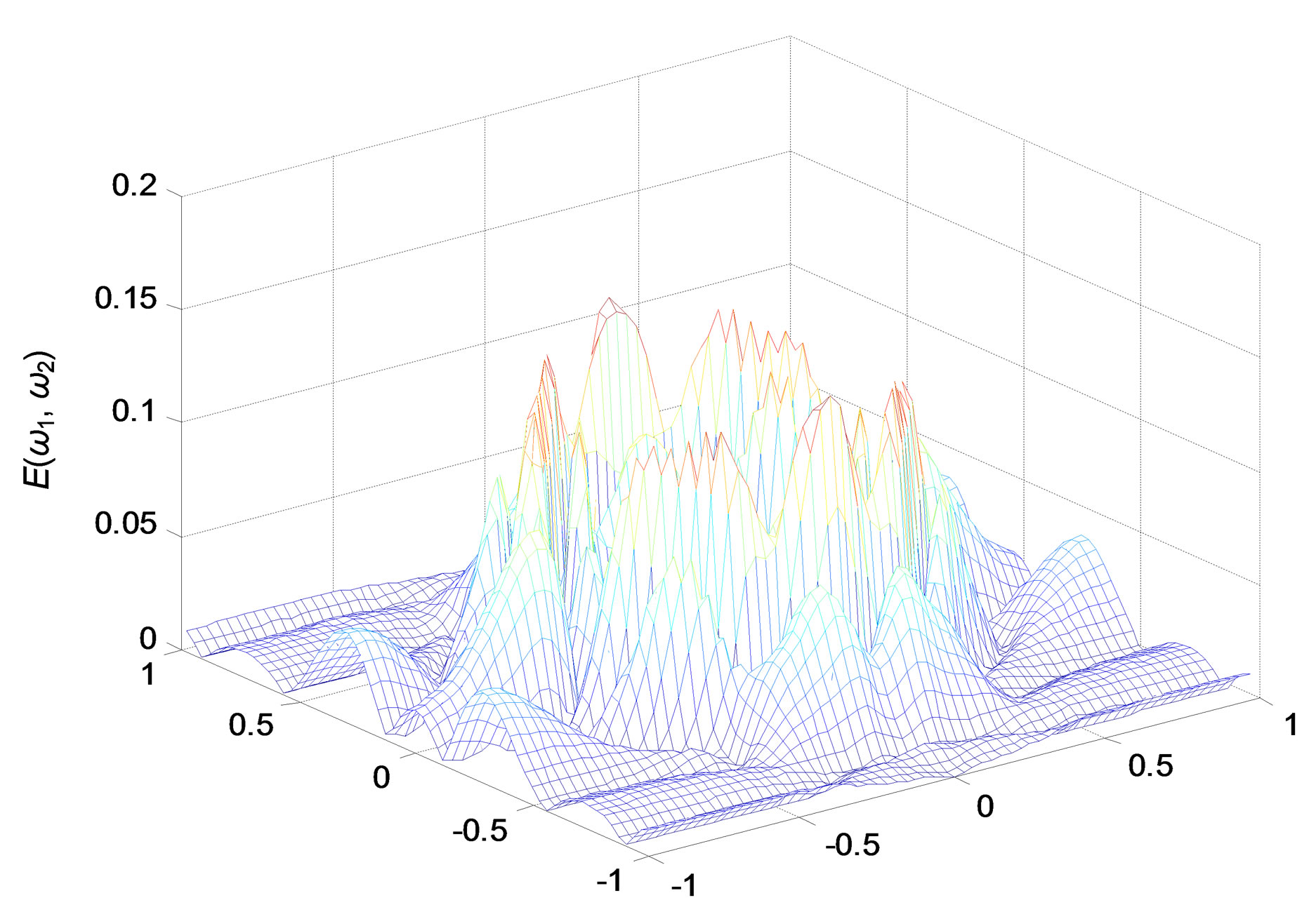
Figure 9. Error specter between original and reduced filter.
 (a)
(a)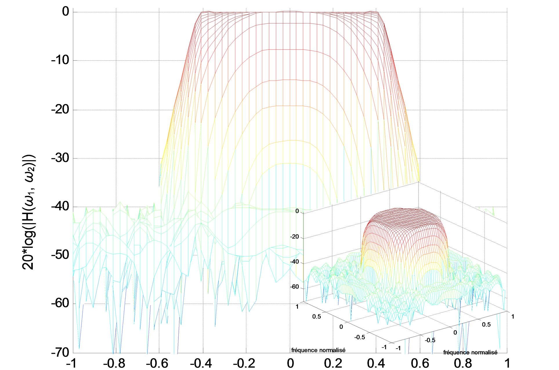 (b)
(b)
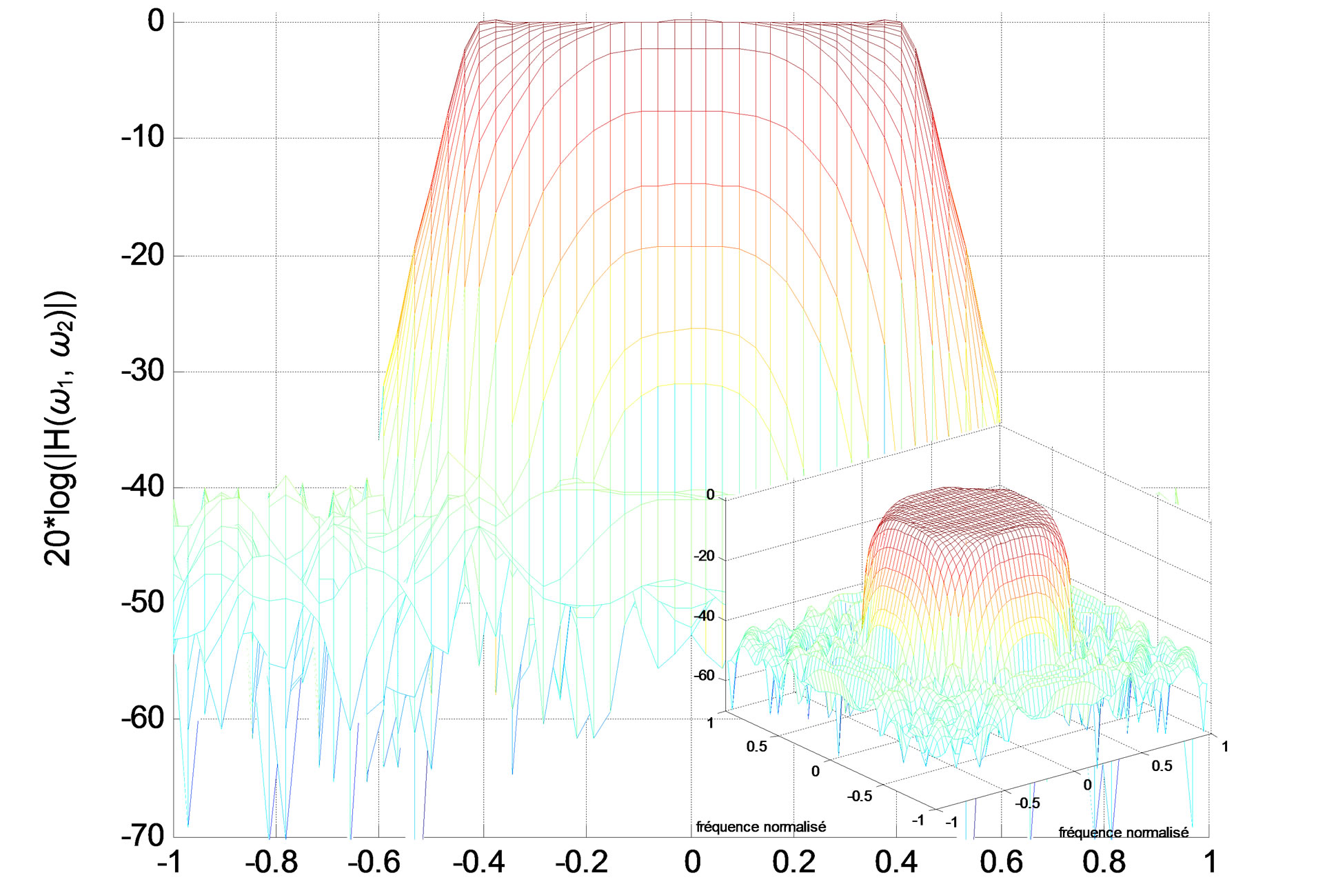
Figure 10. Lowpass IIR filter amplitude responses (in decibels), “X-Z” perspective. (a) Original filter 13 13 (338 coefficients); (b) Reduced-order filter 8 × 8 (128 coefficients).
• In this paper, we attempt to find a design method that solves these problems with conventional methods, such as Prony’s method or Iterative method, which are based on identification ideas. For a zero-phase filter, we divided the support region of the desired impulse response on four regions, then we have synthesized the four filters (one filter in the case where  has a four-fold symmetry) by the Prony method or Iterative method. The result is a linear phase filter which has minimal order (the total num-
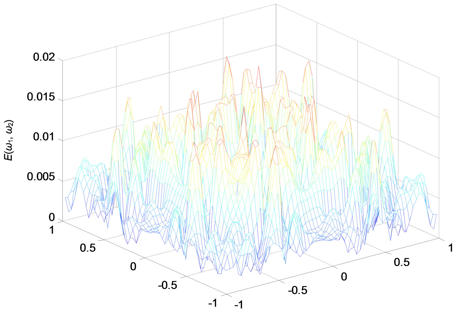
Figure 11. Error specter between original and reduced filter.
ber of coefficients is 200). In the method for Semidefinite Programming (the total number of coefficients is 338), but in this method the stability is guaranteed, with approximately linear phase.
• In the order reduction, we have chosen the method of Quasi-Gramians due to its simplicity. But this method has a disadvantage that it does not preserve the stability in general, but if the system has a separable denominator, the reduced system remains stable, as a filter designed by the SDP method.
REFERENCES
- J. S. Lim, “Two-Dimensional Signal and Image Processing,” Prentice Hall, Upper Saddle River, 1990.
- R. C. Gonzalez and R. E. Woods, “Digital Image Processing,” 3rd Edition, Prentice Hall, Upper Saddle River, 2007.
- W. S. Lu, “Design of Stable 2-D IIR Digital Filters Using Iterative Semidefinite Programming,” Proceedings of ISCAS’00, Geneva, 28-31 May 2000, pp. 395-398.
- W. S. Lu, “A Unified Approach for the Design of 2-D Digital Filters via Semidefinite Programming,” IEEE Transactions on Circuits and Systems, Vol. 49, June 2002, pp. 814-826. doi:10.1109/TCSI.2002.1010036
- T. Kailath, “Linear Systems,” Prentice Hall, Upper Saddle River, 1981.
- K. Premaratne, E. I. Jury and M. Mansour, “An Algorithm for Model Reduction of 2-D Discrete Time Systems,” IEEE Transactions on Circuits and Systems, Vol. 37, No. 9, 1990, pp. 1116-1132. doi:10.1109/31.57600
- S. Y. Kung, B. C. Levi, M. Morf and T. Kailath, “New Results in 2-D Systems Theory, Part II: 2-D State-Space Models-Realization and the Notions of Controllability, Observability, and Minimality,” Proceedings of IEEE, Vol. 65, No. 6, 1977, pp. 945-961.
- E. D. Sontag, “On First Order Equations for MultidimenSional Filters,” IEEE Transactions on Acoustics, Speech and Signal Processing, Vol. 26, No. 5, 1978, pp. 480-482.
- S. Attasi, “Modélisation et traitement des suites à deux indices,” Technical Report 31, INRIA, Le Chesnay, 1975.
- J. L. Shanks, S. Treitel and J. H. Justice, “Stability and Synthesis of Tow-Dimensional Recursive Filters,” IEEE Transactions on Audio and Electroacoustics, Vol. 20, No. 2, 1972, pp. 115-128.
- D. Givone and R. P. Roesser, “Minimization of Multidimensional Linear Iterative Circuits,” IEEE Transactions on Computers, Vol. 22, No. 7, 1973, pp. 673-678. doi:10.1109/TC.1973.5009134
- G. E. Antoniou, P. N. Paraskevopoulos and S. J. Varoufakis, “Minimal State-Space Realization of Factorable 2-D Transfer Function,” IEEE Transactions on Circuits and Systems, Vol. 35, No. 8, 1988, pp. 1055-1058. doi:10.1109/31.1857
- B. C. Moore, “Principal Component Analysis in Linear Systems: Controllability, Observability and Model Reduction,” IEEE Transactions on Automatic Control, Vol. 26, No. 1, 1981, pp. 17-32. doi:10.1109/TAC.1981.1102568
- W. S. Lu, H. Luo and A. Antonio, “Recent Results on Model Reduction Methods for 2-D Discrete Systems,” IEEE Symposium on Circuits and Systems, Atlanta, 12-15 May 1996, Vol. 2, pp. 348-351.
- W.-S. Lu, E. B. Lee and Q. T. Zhang, “Balanced Approximation of Two-Dimensional and Delay Differential Systems,” International Journal of Control, Vol. 46, No. 6, 1987, pp. 2199-2218. doi:10.1080/00207178708934043
- W. Wang, K. Glover, J. C. Doyle and C. Beck, “Model Reduction of LFT Systems,” Proceedings of the 30th IEEE Conference on Decision and Control, Brighton, 11-13 December 1991, pp. 1233-1238. doi:10.1109/CDC.1991.261574
- K. Zhou, J. L. Aravena, G. Gu and D. Xiong, “Two-Dimensional System Model Reduction by Quasi-Balanced Truncation and Singular Perturbation,” IEEE Transactions on Circuits and Systems II: Analog and Digital Signal Processing, Vol. 41, No. 9, 1994, pp. 593-602. doi:10.1109/82.326586
- A. J. Laub, “On Computing Balancing Transformations,” Proceedings of JACC, San Francisco, Vol. 1, Paper FA8- E, 1980.
- H. Luo, W. S. Lu and A. Antoniou, “Numerical Solution of the Two-Dimensional Lyapunov Equations and Application in Order Reduction of Recursive Digital Filters,” IEEE Pacific Rim Conference on Communications, Computers and Signal Processing, Victoria, 19-21 May 1993, pp. 232-235.
- Matlab, “The Matworks™,” Ver. (R2009b).