Journal of Signal and Information Processing
Vol.3 No.3(2012), Article ID:22111,15 pages DOI:10.4236/jsip.2012.33039
A Low Sample Size Estimator for K Distributed Noise
![]()
1Intel Corporation, Hillsboro, USA; 2School of Electrical Engineering and Computer Science, Oregon State University, Corvallis, USA.
Email: eduardo.x.alban@intel.com, *magana@eecs.orst.edu, harry.g.skinner@intel.com
Received May19th, 2012; revised June 20th, 2012; accepted June 30th, 2012
Keywords: Estimation; K Distribution; Mean Square Error; Moments
ABSTRACT
In this paper, we derive a new method for estimating the parameters of the K distribution when a limited number of samples are available. The method is based on an approximation of the Bessel function of the second kind that reduces the complexity of the estimation formulas in comparison to those used by the maximum likelihood algorithm. The proposed method has better performance in comparison with existing methods of the same complexity giving a lower mean squared error when the number of samples used for the estimation is relatively low.
1. Introduction
The estimation of the parameters of a distribution with a limited number of samples available is usually a challenging task. A reduced number of samples constrains the use of the method of moments (MoM) which despite having low complexity has relatively low performance due to its high dependency on the sample size. Prior in [1] presented a study of the minimum number of samples required for the estimation of the K distribution parameters estimators using moments. Estimators with smaller variance based also on moments are usually preferred, though the one based on the maximum likelihood (ML) method is generally the method of choice. Despite the fact that ML estimators are optimal, in some cases they require either the evaluation of uncommon functions or the solution of non-linear equations when no closed-form expressions of them exist.
The K distribution is one of those distributions for which closed-form expressions for all of its ML parameters estimators are not known. The distribution is well known in the radar and sonar community where it has been used to model sea clutter, reverberation and land clutter in synthetic aperture radar ([2-5]). It was introduced by Jakeman and Pusey in [3] for the estimation of the magnitude of scattered radiation. Its extension to a zero-mean symmetric distribution defined over positive and negative values, i.e. double-sided, can easily follow from their derivation [6] and it is given by
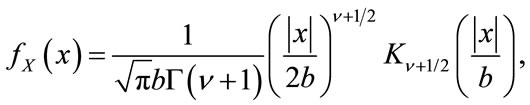 (1)
(1)
with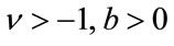 . Furthermore, it has been shown that the distribution is generated by
 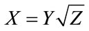 where Y is a zero mean Gaussian random variable with variance b2 and Z is gamma distributed with parameters
  [5].
[5].
Different types of estimators for the K distribution have been proposed that try to overcome the high variance of the MoM and the difficulty in finding ML estimates. Iskander et al. in [7] propose the use of fractional moments which they show produce estimates with lower variance than the MoM. The authors in [8] and [9] propose the use of logarithmic estimators. ML estimates for a limited range of  were presented by Raghavan in [10] based on an approximation of the K distribution using the Gamma distribution. Abraham and Lyons in [11] rely on the MoM with bootstrap to find a better estimator for the shape parameter. The same authors in [12] present an estimator of the shape parameter applied to sonar using a Bayesian adaptation of the MoM with analytical approximations using the gamma distribution (Bayes-MoM-AA), using the bootstrap techniques (BB) and a mixed one with their corresponding performances and trade offs.
Different extensions of the K distribution have been proposed on the literature which have resulted on more tractable expressions for the parameter estimators. Hruska et al. in [13] present estimators for the Homo-dyned K distribution based on the different moments of the distribution. Iskander and Zoubir in [14] introduce a generalized version of the distribution that the authors named as the Generalized Bessel K distribution (GBK) thanks to which in [7] they were able to find a ML closed-form expression for the parameter b of the K distribution in terms of . The distribution results from a generalized Gamma random variable with scale parameter that is also generalized Gamma distributed. The probability density function (pdf) is given by
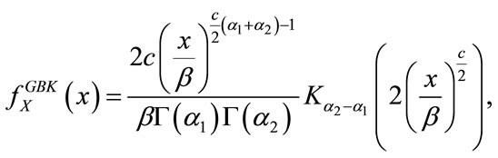 (2)
(2)
with . It is understood that
  . The double-sided K distribution can be derived from the GBK as
 (3)
(3)
Other methods rely heavily on numerical methods to find the parameters estimates. They make use of iterative methods such as the Expectation-Maximization as in [15] and [16], 2-D maximizations as in [17], neural networks as in [8] and [18] or non-linear techniques, among others. These methods are robust albeit computationally expensive, which make real time applications infeasible.
In this paper we derive an estimator that retains the simplicity of the method of moments with comparable computational requirements but has better performance when a small number of samples are available. The method is compared with other methods of the same complexity through simulations.
The rest of the paper is organized as follows: In Section 2 we review some of the existing estimation methods. In Section 3, the derivation of the new estimation method is presented. Section 4 presents simulation results. Finally, Section 5 presents some conclusions.
2. Parameter Estimation Review
In this section we briefly review some of the estimators that have been proposed for the K distribution, which will be compared with our proposed method in a later section. Specifically, we proceed to find the estimators for the two parameters  and b that define the doublesided distribution.
2.1. Method of Moments
The method of moments (MoM) computes the parameters of a distribution by finding expressions in terms of its moments. The moments are then replaced by their corresponding empirical ones computed from the sample set.
The moments of a K distributed random variable X are defined as  and they are computed as follows:
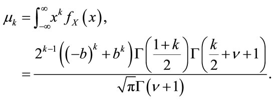 (4)
(4)
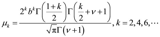
We notice that whenever k is an odd integer  and when k is an even integer the moments are given by
Then, it follows that the second moment (the variance for zero-mean distributions) is given by
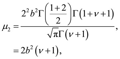 (5)
(5)
and the fourth moment by
Thus, the kurtosis which is defined as  is given by
It follows that the estimators of  and b are found to be
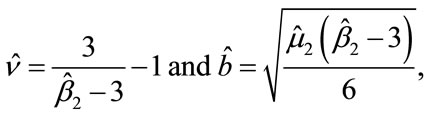 (6)
(6)
respectively, where  is the second empirical moment of the data and
  is the empirical kurtosis.
The estimators are computationally inexpensive and easy to implement but they depend heavily on the number of samples available. A small sample set causes the variance of the estimator to increase to levels that make the estimation unreliable as it is seen on Figure 1. The figure shows MoM estimates and their variances for parameters  and
and  over 5000 independent trials as a function of the sample size.
2.2. Fractional Moments
Iskander in [19] noticed that fractional moments produce estimates with lower variances. His method proposes the use of the ratio:
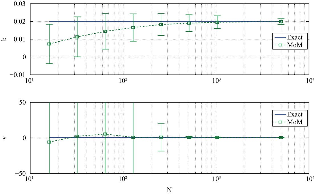
Figure 1. Parameter estimation (MoM)  = 0.5, b = 0.02.
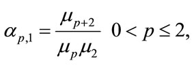 (7)
(7)
which in the case of the type of K distribution studied here comes with the restriction . Replacing the expression with the moments formula given in (4), applying the properties of the gamma function and after some simplifications, we find that the expression for the double-sided K distribution turns out to be
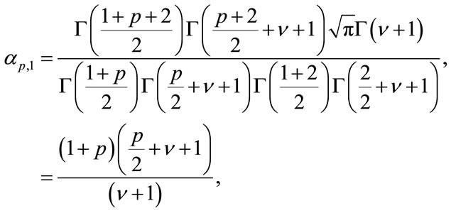 (8)
(8)
which is independent of b. Then, the parameter  can be easily estimated using the corresponding empirical ratio, namely
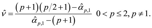 (9)
(9)
The value of b can be estimated using the empirical second moment or any other moment since they establish a relation between b and .
.
2.3.  Estimation
Blacknell and Tough in [9] proposed an estimator of  based on
  which gives a comparable accuracy with the fractional moments estimators among others. They noticed that setting
  leads to simple expressions for the estimator of
  of the one-sided K distribution. We proceed with the derivation of the estimate that corresponds to the double-sided K distribution. This derivation follows the one given in [9], though in this case it is easily seen that setting
  gives an estimate that does not have
  as an argument of any
 ,
,  or any other exotic function. We also notice that the distribution is zero-mean and symmetric around the mean, therefore it makes sense to work with the absolute values since the logarithm of negatives values is not defined.
Now,
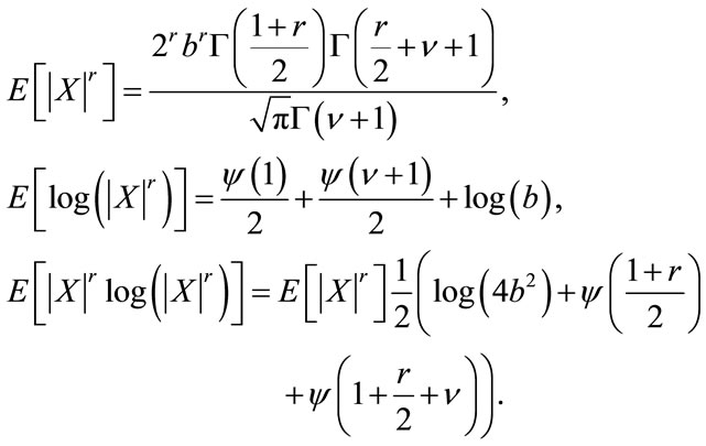 (10)
(10)
Setting r = 2 in the previous results we evaluate the following expression:
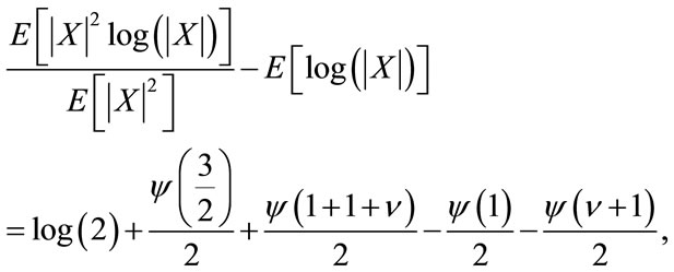 (11)
(11)
since  and
and
 . Hence,
 (12)
(12)
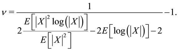
The estimate  is obtained by replacing the expected values by their corresponding empirical estimates.
2.4. Maximum Likelihood Estimation
Maximum Likelihood (ML) estimation is one of the most reliable estimator even when only a limited number of samples exist. Also, the ML estimator is asymptotically unbiased and it attains the Cramer-Rao lower bound asymptotically better than any other unbiased estimator. Though the ML estimator performs better than other methods, its high complexity prevents its use when limited computational capabilities are available.
The ML estimator results from the maximization of the likelihood or the log-likelihood function, whichever gives a more tractable expression. In the case of the K distribution the log-likelihood l is preferred and it is given by
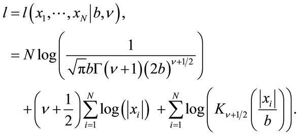 (13)
(13)
The parameters estimators are obtained by maximizing the log-likelihood function, but it is evident from its partial derivatives
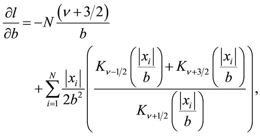 (14)
(14)
and
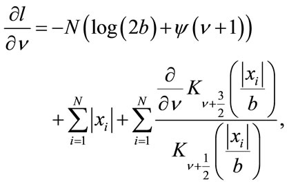 (15)
(15)
that finding closed-form solutions for both parameters is a difficult task. In fact, closed-form expressions cannot be directly obtained from them [7,9,10,15,17].
Iskander et al. in [7] derived a closed-form expression for one of the parameters by first finding an expression for the parameter  from the generalized Bessel K distribution
 (16)
(16)
where  is the digamma function. The parameter b of the double-sided K distribution can easily be obtained following the relationship given in (3). Replacing the corresponding values
 , it follows that
 (17)
(17)
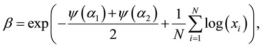
which turns out to be a non-linear function of . The authors also found from the maximization of the likelyhood function that
 (18)
(18)
where
 (19)
(19)
for the generalized Gamma distribution. The maximum likelihood estimates can then be found using the expressions just presented and the equivalence in (3) for the double-sided K distribution. Although there exists a closed-form expression for one of the parameters, we are still required to use computationally intensive methods to find both parameters estimates.
In [7] the maximum likelihood estimates are found using a cubic spline interpolation. In [15] the iterative method known as the Expectation-Maximization is employed. Finally in [8] and [20] neural networks are used. This has lead us to investigate a new estimate that retains the simplicity of the estimators previously presented which yields accurate estimates when we only have access to small sample sets of the process.
2.5. Cramer-Rao Lower Bound
The Cramer-Rao lower bound (CRLB) gives a bound on the performance of an estimator. Specifically, it tells us about the minimum value that the variance of an unbiased estimator can achieve. In other words,
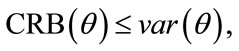 (20)
(20)
where  is the estimator.
The CRLB is given by
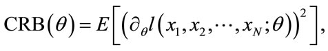 (21)
(21)
where  is the log-likelihood function. Deriving a closed-form expression of the CRLB for the K distribution would be a daunting task but for specific parameters of the distribution. Kay and Hu in [21] have also proposed a method to compute the bound using the characteristic equation. For the purpose of comparing the different estimation methods we proceed to evaluate the CRLB numerically.
3. New Estimator
We propose an approximate method that leads us to a more tractable expression for the estimation of the K distribution parameters. This approximation turns out to have better performance than others for a low number of samples.
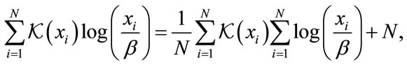
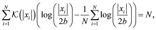
We now proceed to derive estimators that have as a starting point an expression found in [7] that results from the maximization of the log-likelihood of the GBK distribution. The authors found that maximizing the loglikelihood gives the following expression:
 (22)
(22)
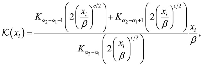
where
 (23)
(23)
Since standalone expressions derived from the previous equations are not known, using numerical methods as in [7] are the only methods to find the estimators.
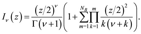
We notice that the presence of the modified Bessel function of the second kind,  adds complexity to the derivation of estimators. Thus, it is more convenient to express
  in terms of well known functions since it eases the burden of finding the estimators.
Now, it follows that for a large argument the modified Bessel function K can be approximated by [22]
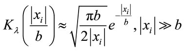 (24)
(24)
where the approximation corresponds to an equality regardless of its argument when .
.
An expression for the estimator of b for the doublesided distribution can be obtained by first using the equivalence defined in (3) and the approximation (24) in (23). It follows that
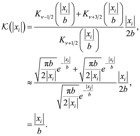 (25)
(25)
Now, let 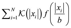 then
then
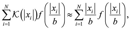 (26)
(26)
holds whenever  is a monotonic function. Then, assuming that only a small fraction of the data does not satisfy the condition
  and using (25) on (22) we have that
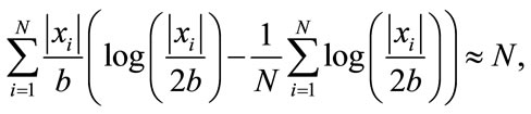
which holds since the log function is monotonic.
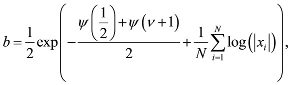
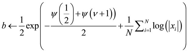
It is now easy to show in a few steps that the estimator of b is given by
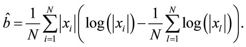 (27)
(27)
The expression for  just derived does not depend on
 , it is computationally inexpensive and it can be implemented using a fairly simple architecture.
The parameter  can be easily estimated from any of the moments and the estimate of b just derived. One of the options is to use the second moment as follows:
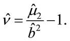 (28)
(28)
The estimators assume that the ’s values that are larger than b outnumber those that are not, because this ensures that the actual value of the K function is mostly dominated by the approximation (24). On the one hand, if b is infinitesimally small the condition is easily met since almost all
  are larger than it. On the other hand, if b is large, our estimators still perform well whenever N is small since only a fraction of the
 ’s would be smaller than b and the approximation holds.
Estimator Bias
The bias of the estimator is given by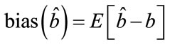 . Now,
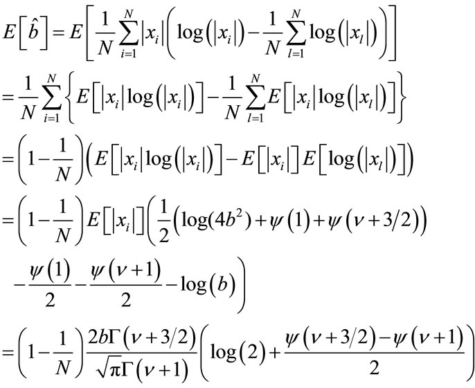
Then, the bias is given by
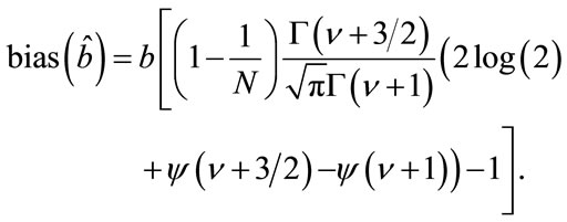 (29)
(29)
The asymptotic bias can be computed from the previous expression as
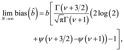 (30)
(30)
where it can be easily seen that 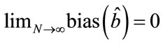 only when
 . Therefore, the estimator just derived is not unbiased or asymptotically unbiased, except for
 .
.
The accuracy of the estimator can be improved by subtracting the bias from the estimator. However, by doing so we end up with the same situation as before, even though without the modified Bessel function of the second kind. This is because the bias of b depends on the value of . Therefore, in order to find the estimates we will need an iterative process to find the values which increases the computational requirements of the estimators.
In the next section the performance of this estimator and the ones described on the previous section are quantified.
4. Simulation Results
A series of Monte Carlo simulations were carried out to evaluate the performance of the estimators. The estimation methods were applied over 5000 realizations of a K distributed process and their performances were analyzed using as a measure the mean-square error. For compareson, a maximum likelihood was computed using a onedimensional search for the parameter  with (17) substituting the corresponding value in (19). Also, the Cramer-Rao lower bound (CRLB) was evaluated numerically to compare it with the others estimators.
We first analyze the performance of the estimators in terms of the number of samples available. The analyses are constrained to take on parameters with small values,  and
and  which does not limit its applicability since most of the known processes fall within those ranges. Figures 2 and 3 show some of the results for a K distributed random process with parameters
 ,
,  and
and ,
, . Comparing with the other methods, our estimator outperforms them whenever N is small,
  for the cases shown here. We notice that when N is large, the performance of our estimator does not improve as the other methods do, being outperformed by them. This is not an unexpected result since our estimator is based on an approximation that does not guarantee the asymptotic unbiasedness of the estimator for all values of
 . We also notice that for small N our estimator performs similar to the maximum likelihood estimator with some values giving a slightly better performance due to the inaccuracies of the onedimensional search that depends on the choices of the grid spacing.
The behavior of the estimators in terms of  for the range −1 to 1.5 is also analyzed. We present here simulation results with
  and N = 32, 64, 128, 256, 512. Figures 4, 5 and 6 show the estimators when N = 32, 64, 128. The results confirm that our estimators are more consistent and perform better than the others except for
 , where the fractional MoM and the
  perform slightly better. The simulations show that our method performs quite well for parameters
  and
and . This does not limit the scope of the estimator since there is a wide range of K distributed processes with parameters inside that range. The proposed estimator together with the maximum likelihood estimator (MLE) are the ones whose mean-squared error is closer
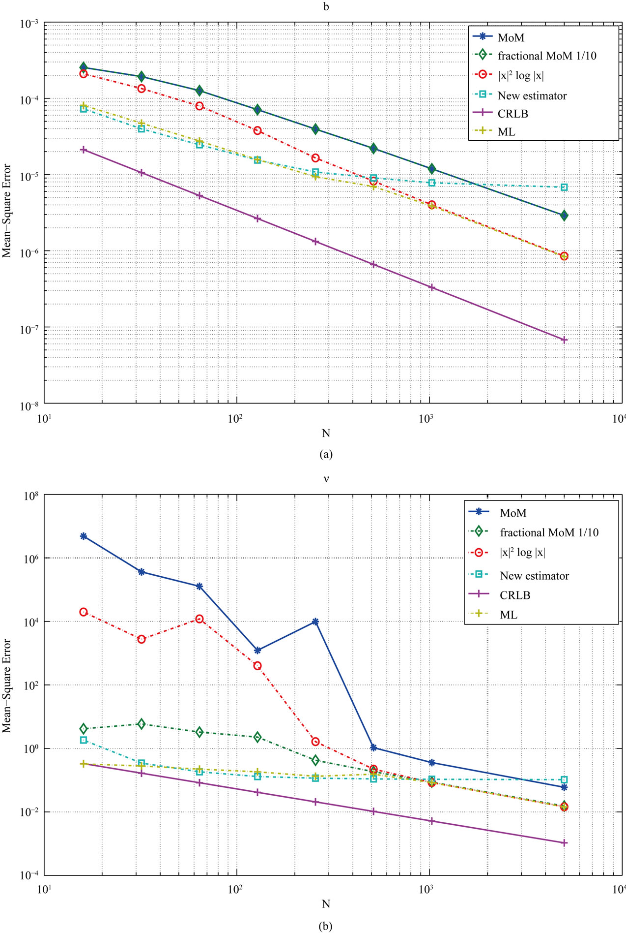
Figure 2. MSE estimators comparison:  = 0.5, b = 0.02. (a) Estimators of b; (b) Estimators of
 .
.
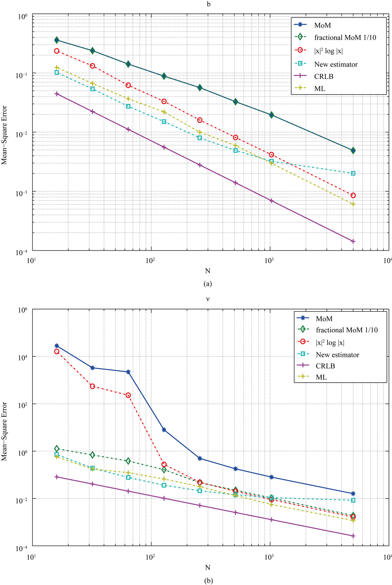
Figure 3. MSE estimators comparison:  = −0.2, b = 0.8. (a) Estimators of b; (b) Estimators of
 .
.
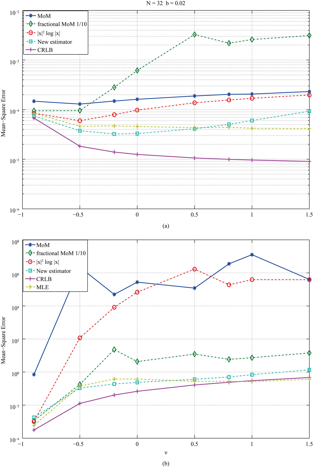
Figure 4. MSE estimator comparison: N = 32, b = 0.02. (a) Estimators of b; (b) Estimators of .
.
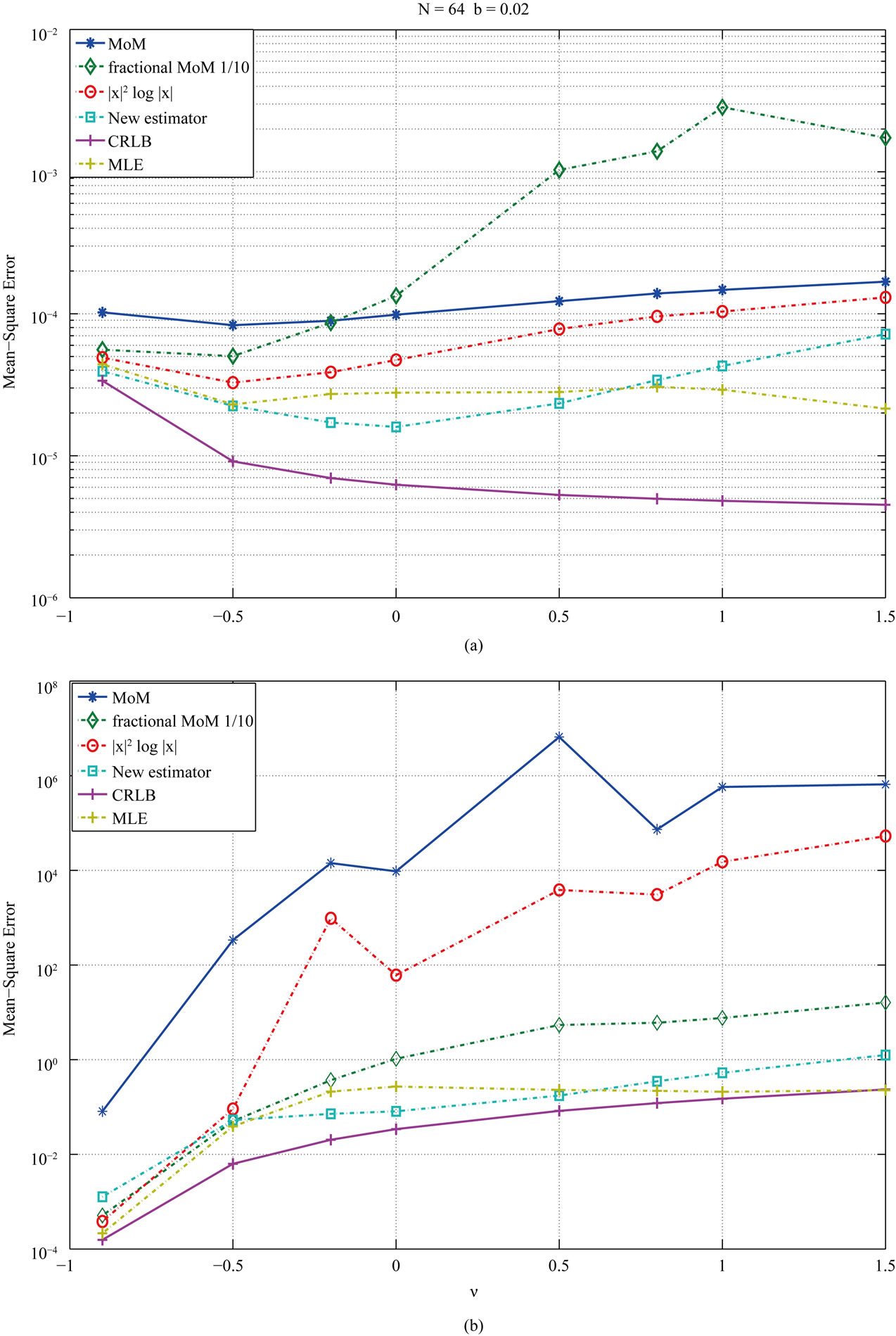
Figure 5. MSE estimator comparison: N = 64, b = 0.02. (a) Estimators of b; (b) Estimators of .
.
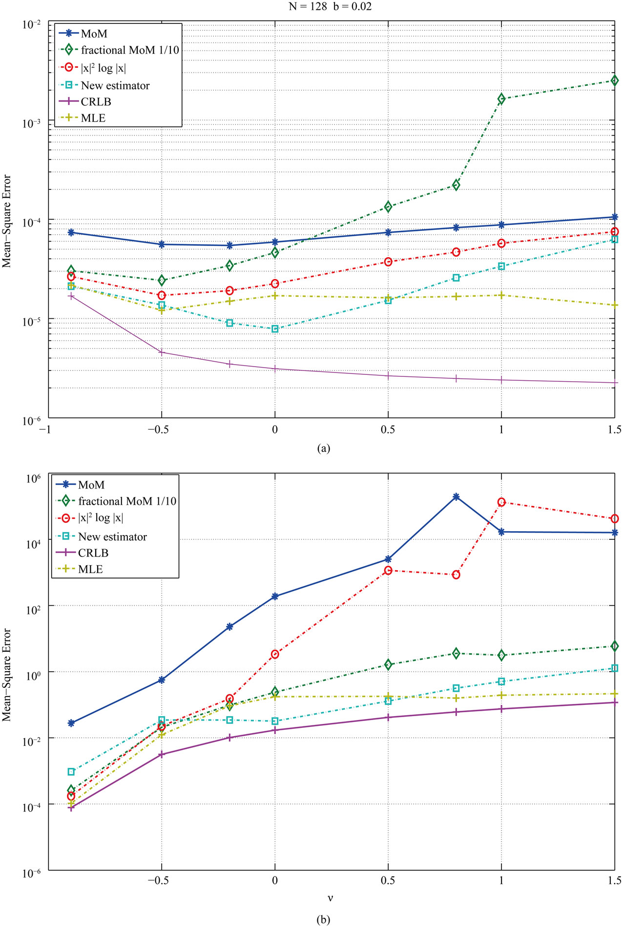
Figure 6. MSE estimator comparison: N = 128, b = 0.02. (a) Estimators of b; (b) Estimators of .
.
to the CRLB when N is small. In general, the MLE is closer to the CRLB for all values of N.
The performance of the other estimators improves as the number of samples available for the estimation increases, as it is seen on Figure 7 for N = 256. Specially the  outperforms the rest but for some values in which our estimators still outperform them.
In [9], it was argued that the estimator based on  comes as a natural limit of the fractional moments estimator of [19], this turns out to be true when the number of samples N is large, where how large N should be depends on the parameters
  and b, but not when N is small as it is shown in the figures. The results confirm that the proposed estimator outperforms other estimators that are comparable in terms of complexity and computational requirements.
5. Computational Complexity
In this section we present an analysis of the computational complexities of the estimators presented in the previous sections. Specifically, we focus on the analysis for the estimators of the parameter  referring to the expressions given in (6), (9), (12), (17), (18), (19), (27) and (28).
The evaluation of the estimators is straight forward except in the case of the MLE estimator which, as we mentioned before, needs to be evaluated through a onedimensional search. We use an iterative method to solve the one-dimensional search where a set of values is applied to the respective equations until the one that better satisfies the equations is found. Specifically, the MLE estimator is computed with the following algorithm:
For each 
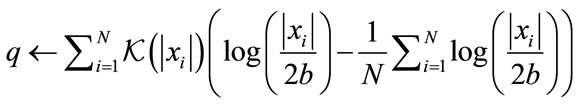
If q ≈ 0 then Return 
end if end for where V is the set of all points that form the grid over which the one-dimensional search is done and  is equal to (19). Let
  be the average number of iterations the algorithm needs to compute the estimate
 , then the number of operations is given by
  where
where  is the number of operations per iteration. The value of
  depends on the grid size and its spacing. Limiting the range of values where to search would greatly reduce the grid size, otherwise,
  could be too large to be implemented on real time applications.
Table 1 summarizes the number of operations that each estimation method requires. In the case of the MLE estimator the table shows the number of operations per iteration. In the following analysis we ignore the complexity that the evaluation of the digamma function, exponential function and the square root requires since if they are evaluated in an estimator, they are only done once. In the case of the absolute value, the implementation only requires a check on the sign so overall in comparison with operations such as multiplications and additions its contribution to the computational complexity can be ignored. We also notice that any quantity raised to the second power is simply a multiplication with itself. Therefore the analysis reduces to the quantification of additions, multiplications, divisions, the evaluation of logarithm and the modified Bessel function of the second kind .
.
The modified Bessel function of the second kind is given by
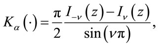 (31)
(31)
where  can be expressed as [23]
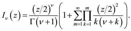 (32)
(32)
The evaluation of  can be conducted using a forward recurrence following the method described in [23], but for the matter of quantifying its computational complexity we truncate the infinite series (32) to some
  that defines the accuracy of the computed value. Then, the truncated series is given by
 (33)
(33)
The number of operations that contributes largely to the evaluation of  using the truncated series is shown in Table 2.
Now, we can quantify the complexity of the estimators in terms of basic operations such as additions , multiplications
 , divisions
  as it is summarize in Table 3.
The highest complexity is due to the number of multiplications and divisions. Therefore we quantified the computational complexity in terms of both operations. In terms of multiplications, the complexity for the MLE is given by 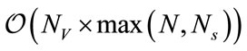 and for the rest of the estimators including the new method is given by
 . In terms of divisions, the complexity of the MLE is
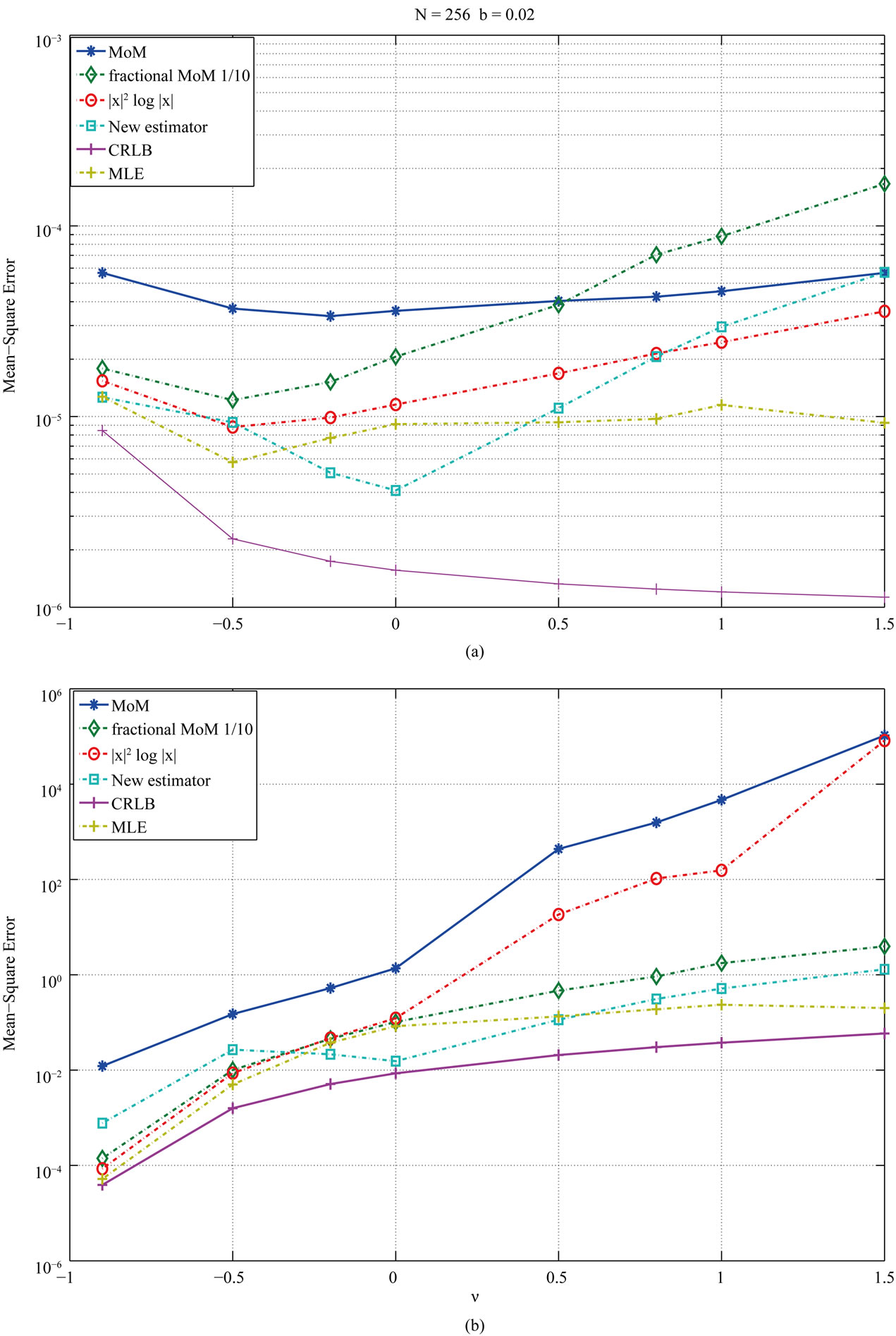
Figure 7. MSE estimator comparison: N = 256, b = 0.02. (a) Estimators of b; (b) Estimators of .
.
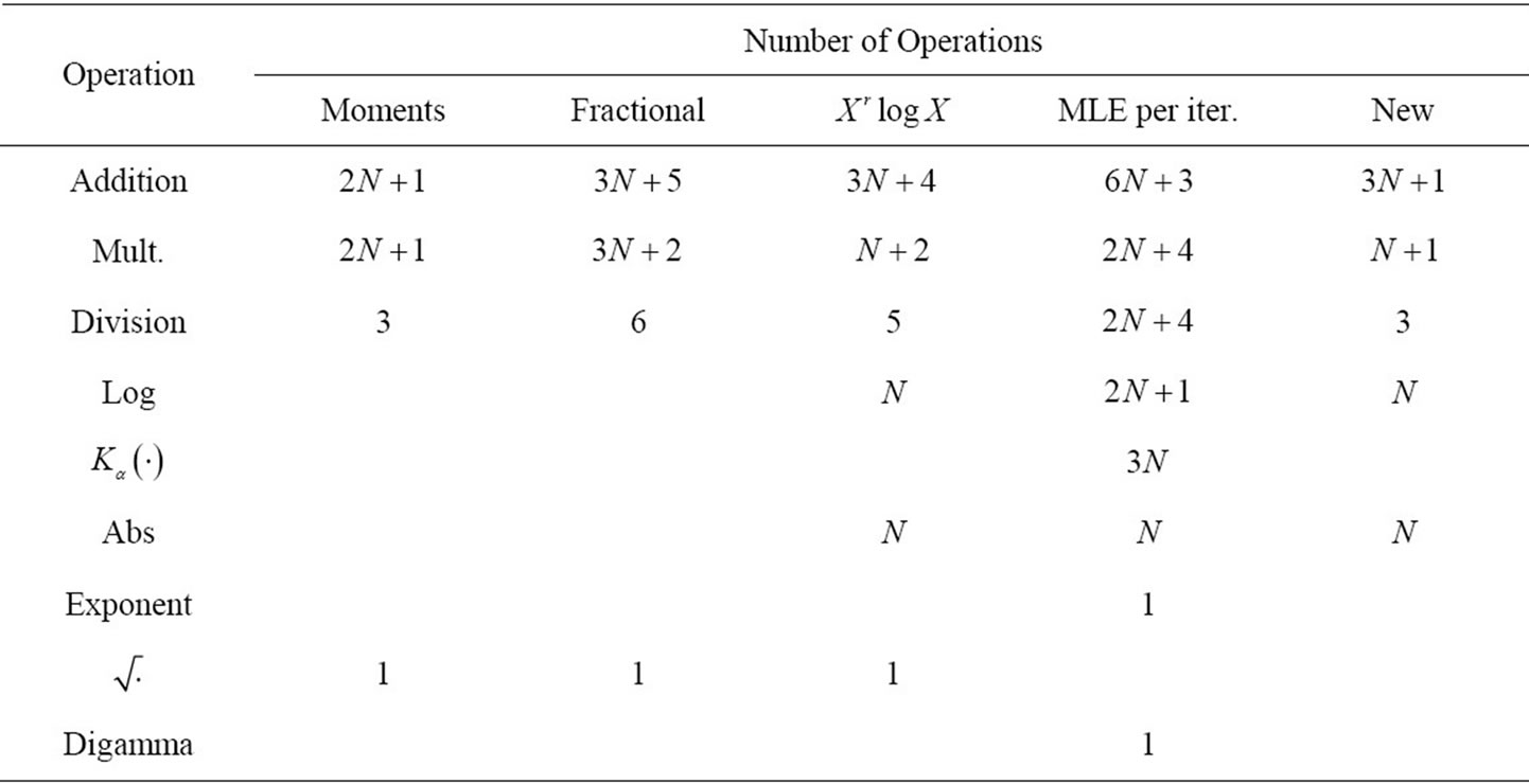
Table 1. Number of operations of estimators.
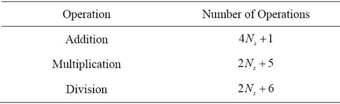
Table 2. Number of operations of a truncated modified Bessel function of the second kind.
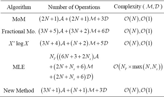
Table 3. Complexity of estimators.
 and for the new and other estimators is
 .
.
The new method has been proved to have a computational complexity that is comparable with estimators based on moments but low in comparison with the MLE.
6. Conclusion
In this paper we have derived a new estimation method for the K distribution. The method provides an improved performance over existing techniques when only a limited number of samples is available. It has been shown through Monte Carlo simulations that the method produces estimates with smaller variance than others while maintaining their simplicity and computational requirements low. The performance of the proposed estimator is comparable to the maximum-likelihood without the complexity that this one requires.
7. Acknowledgements
We would like to thank the Intel Corporation for funding this research work.
REFERENCES
- M. K. Prior, “Estimation of K-distribution shape parameter from sonar data: Sample size limitations,” IEEE Journal of Oceanic Engineering, vol. 34, no. 1, 2009, pp. 45-50. Hdoi:10.1109/JOE.2008.2008040
- C. J. Baker, “K-distributed coherent sea clutter,” IEEE Proceedings F Radar and Signal Processing, vol. 138, no. 2, 1991, pp. 89-92. Hdoi:10.1049/ip-f-2.1991.0014
- E. Jakeman and P. Pusey, “A model for Non-Rayleigh sea echo,” IEEE Transactions on Antennas and Propagation, vol. 24, no. 6, 1976, pp. 806-814. Hdoi:10.1109/TAP.1976.1141451
- C. J. Oliver, “Optimum texture estimators for SAR clutter,” Journal of Physics D: Applied Physics, vol. 26, no. 11, 1993, p. 1824. http://stacks.iop.org/0022-3727/26/i=11/a=002=0pt
- D. A. Abraham and A. P. Lyons, “Novel physical interpretations of K-distributed reverberation,” IEEE Journal of Oceanic Engineering, vol. 27, no. 4, 2002, pp. 800-813. Hdoi:10.1109/JOE.2002.804324
- S. Kay, “Representation and generation of non-Gaussian Wide-Sense Stationary Random processes with arbitrary PSDs and a class of PDFs,” IEEE Transactions on Signal Processing, vol. 58, no. 7, 2010, pp. 3448-3458. Hdoi:10.1109/TSP.2010.2046437
- D. R. Iskander, A. M. Zoubir and B. Boashash, “A method for estimating the parameters of the K distribution,” IEEE Transactions on Signal Processing, vol. 47, no. 4, 1999, pp. 1147-1151. Hdoi:10.1109/78.752614
- M. Jahangir, D. Blacknell and R. G. White, “Accurate approximation to the optimum parameter estimate for K-distributed clutter,” IEEE Proceedings—Radar, Sonar and Navigation, vol. 143, no. 6, 1996, pp. 383-390. Hdoi:10.1049/ip-rsn:19960842
- D. Blacknell and R. J. A. Tough, “Parameter estimation for the K-distribution based on [z log(z)],” IEEE Proceedings—Radar, Sonar and Navigation, vol. 148, no. 6, 2001, pp. 309-312. Hdoi:10.1049/ip-rsn:20010720
- R. S. Raghavan, “A method for estimating parameters of K-distributed clutter,” IEEE Transactions on Aerospace and Electronic Systems, vol. 27, no. 2, 1991, pp. 238-246. Hdoi:10.1109/7.78298
- D. A. Abraham and A. P. Lyons, “Bootstrapped K-distribution parameter estimation,” OCEANS 2006, Boston, 18-21 September 2006, pp. 1-6. Hdoi:10.1109/OCEANS.2006.306983
- D. A. Abraham and A. P. Lyons, “Reliable methods for estimating the K-distribution shape parameter,” IEEE Journal of Oceanic Engineering, vol. 35, no. 2, 2010, pp. 288-302. Hdoi:10.1109/JOE.2009.2025645
- D. P. Hruska and M. L. Oelze, “Improved parameter estimates based on the Homodyned K distribution,” IEEE Transactions on Ultrasonics, Ferroelectrics, and Frequency Control, vol. 56, no. 11, 2009, pp. 2471-2481. Hdoi:10.1109/TUFFC.2009.1334
- D. R. Iskander and A. M. Zoubir, “Estimating the parameters of the K-distribution using the ML/MoM approach,” Proceedings of 1996 IEEE TENCON. Digital Signal Processing Applications, Perth, 26-29 November 1996, pp. 769-774.
- W. J. J. Roberts and S. Furui, “Maximum likelihood estimation of K-distribution parameters via the expectation-maximization algorithm,” IEEE Transactions on Signal Processing, vol. 48, no. 12, 2000, pp. 3303-3306. Hdoi:10.1109/78.886993
- P.-J. Chung, W. J. J. Roberts and J. F. Bohme, “Recursive K-distribution parameter estimation,” IEEE Transactions on Signal Processing, vol. 53, no. 2, 2005, pp. 397- 402. Hdoi:10.1109/TSP.2004.840811
- I. R. Joughin, D. B. Percival and D. P. Winebrenner, “Maximum likelihood estimation of K distribution parameters for SAR data,” IEEE Transactions on Geoscience and Remote Sensing, vol. 31, no. 5, 1993, pp. 989-999. Hdoi:10.1109/36.263769
- A. Mezache and F. Soltani, “A new approach for estimating the parameters of the K-distribution using fuzzyneural networks,” IEEE Transactions on Signal Processing, vol. 56, no. 11, 2008, pp. 5724-5728. Hdoi:10.1109/TSP.2008.929653
- D. R. Iskander and A. M. Zoubir, “Estimation of the parameters of the K-distribution using higher order and fractional moments [radar clutter],” IEEE Transactions on Aerospace and Electronic Systems, vol. 35, no. 4, 1999, pp. 1453-1457. Hdoi:10.1109/7.805463
- M. P. Wachowiak, R. Smolikova, J. M. Zurada and A. S. Elmaghraby, “Estimation of K distribution parameters using neural networks,” IEEE Transactions on Biomedical Engineering, vol. 49, no. 6, 2002, pp. 617-620. Hdoi:10.1109/TBME.2002.1001977
- S. Kay and C. Xu, “Crlb via the characteristic function with application to the K-distribution,” IEEE Transactions on Aerospace and Electronic Systems, vol. 44, no. 3, 2008, pp. 1161-1168. Hdoi:10.1109/TAES.2008.4655371
- M. Abramowitz and I. A. Stegun, “Handbook of Mathematical Functions: with Formulas, Graphs, and Mathematical Tables,” In: M. Abramowitz and I. A. Stegun, Eds., Dover Books on Advanced Mathematics, Dover Publications, New York, 1965.
- S.-C. Zhang and J.-M. Jin, “Computation of special functions,” Wiley, New York, 1996. http://books.google.com/books?id=ASfvAAAAMAAJ =0pt
NOTES
*Corresponding author.