International Journal of Geosciences
Vol.06 No.05(2015), Article ID:56337,5 pages
10.4236/ijg.2015.65038
ESMD Method for Frequency Distribution of Tank Surface Temperature under Wind Effect
Jinliang Wang1,2, Xianshui Fang1
1College of Science, Qingdao Technological University, Qingdao, China
2Oceanic Telemetry Engineering and Technology Research Center, State Oceanic Administration, Qingdao, China
Email: wangjinliang0811@126.com, 1228629058@qq.com
Copyright © 2015 by authors and Scientific Research Publishing Inc.
This work is licensed under the Creative Commons Attribution International License (CC BY).
http://creativecommons.org/licenses/by/4.0/


Received 24 April 2015; accepted 12 May 2015; published 15 May 2015
ABSTRACT
Due to the poor understanding of the small-scale processes at the air-water interface, some lab experiments are done in a water tank by infrared techniques. With the help of ESMD method, the stochastic temperature sequences extracted from the infrared photographs are decomposed into several empirical modes of general periodic forms. The corresponding analyses on the modes reveal that, within certain limits, both spatial and temporal frequencies increase along the wind speed. As for the amplitudes, the existence of wind may result in fold increasing of their values. In addition, when the wind speed is added from 4 m/s to 5 m/s, both frequency and amplitude of the surface temperature decrease and it implies an enhanced mixing and a weakened temperature gradient under the force of wind blowing.
Keywords:
Extreme-Point Symmetric Mode Decomposition (ESMD), Surface Temperature, Time-Frequency Distribution, Wind, Wave Tank Experiment

1. Introduction
The extreme-point symmetric mode decomposition (ESMD) method [1] [2] can be seen as a new alternate of the well-known Hilbert-Huang transform [3] . Due to the advantages of ESMD method in de-trending, abnormity diagnosis and time-frequency analysis, an effective usage is anticipated in scientific exploration. In fact, as our researches concerned, in addition to the feasibility of application in climate data analysis [4] , it has already been used successfully in air-sea flux study [5] . In this article, we use it to investigate the small-scale temperature variation at air-water interface.
Just as mentioned by Veron et al. in 2008 [6] , while attention has historically focused on larger-scale longer- term phenomena, the mechanisms involved in small-scale mixing still remain rather poorly understood. With the difference between kinematics viscosity and thermal diffusivity being almost one order of magnitude, the heat transferring is usually impacted by the dynamic processes and the thermal sub-layer is typically within the viscous sub-layer. Therefore, the infrared thermal techniques appear promising in this regard. The results in [6] and [7] for the effects of wind speed on temperature variations are obtained by field observations at sea, where there are many uncontrollable factors. Here we check them in a lab.
2. Lab Experiments
The experiments are done on the morning of Sept. 12,
3. ESMD Decomposition
Take the 60th infrared photograph obtained by the second experiment (accords to wind speed U = 3 m/s) as an example. Its 160th column forms a one-dimensional stochastic spatial sequence with 240 points which can be considered by ESMD method. This new method can help us to reveal the detailed variation of the surface temperature. By executing the ESMD programs it yields three modes together with a remainder R which is an optimal global mean fitting curve in the sense of least squares (see Figure 1). Correspondingly, the direct-inter- polating approach (the second part of ESMD method) yields a distribution of spatial frequencies for these modes (see Figure 2). Certainly, that of amplitudes can be also outputted and its figure is omitted here. We note that the variations of spatial frequencies along the distance in our figure are much more intuitive than those given by the Hilbert spectrum in [3] .
4. Distributions for Spatial Frequency and Amplitude
To get a relatively objective statistic result we choose the 40th, 45th, 50th, 55th and 60th infrared photographs to do the decompositions. For the no wind case, their optimal sifting times are 5, 5, 5, 4 and 5 which yield three empirical modes for each of them, that is, each ruleless stochastic spatial sequence has now been divided into 3 subsequences of general periodic forms with different scales. Correspondingly, the spatial frequencies for the first modes of them are 3.1801, 2.9114, 3.05696, 3.0317 and 3.0401 with unit “cm−1” separately. They have a mean value 3.0401 cm−1 which can be seen as the highest frequency of temperature variation in the sense of statistics. At this time, one can also get the amplitudes 0.0086, 0.0087, 0.0081, 0.0090 and 0.0100 with a mean value 0.0089 (with unit “˚C”). In the same way we get those for the other two modes. Under the similar settings, the repetition of the above processing also yields the statistic results for the cases 3 m/s, 4 m/s and 5 m/s. It follows from Figure 3 that, as the wind speed increases (expect the case of 5 m/s), the spatial frequencies at dif- ferent scales increase in a certain extent. Relative to the no-wind case the mean increments of those for 3 m/s
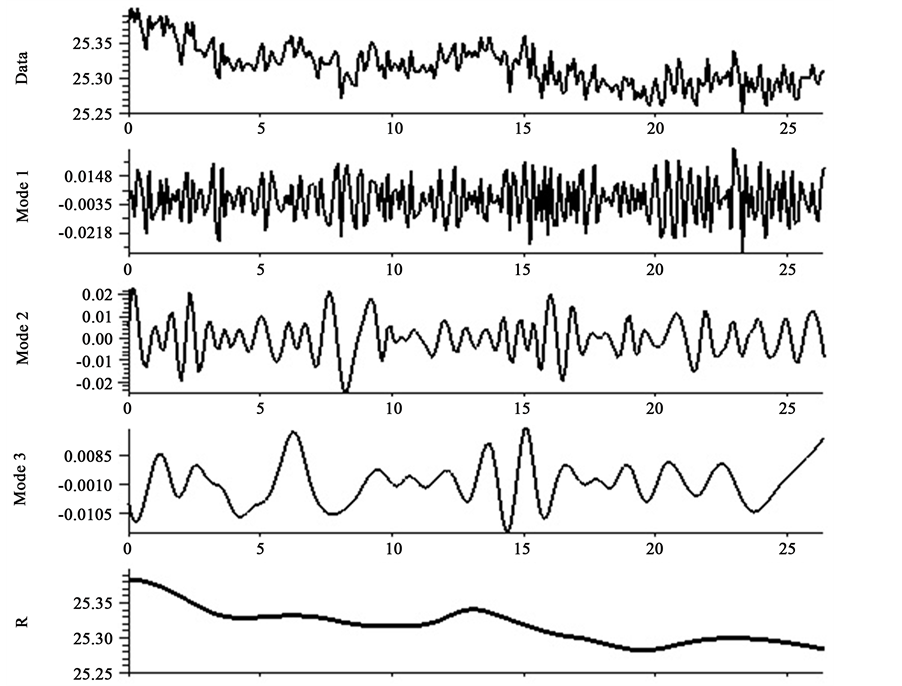
Figure 1. The decomposition result given by ESMD method with 5 sifting times, here the horizontal axis stands for the distance with unit “cm”.
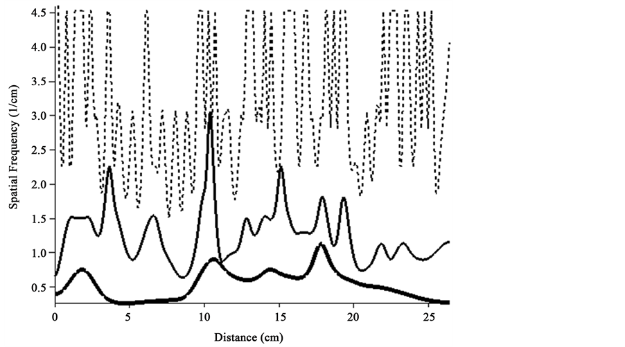
Figure 2. The distribution of spatial frequencies for the 3 modes (from above to below, the curves stands for that of mode 1 mode 2 and mode 3 separately).
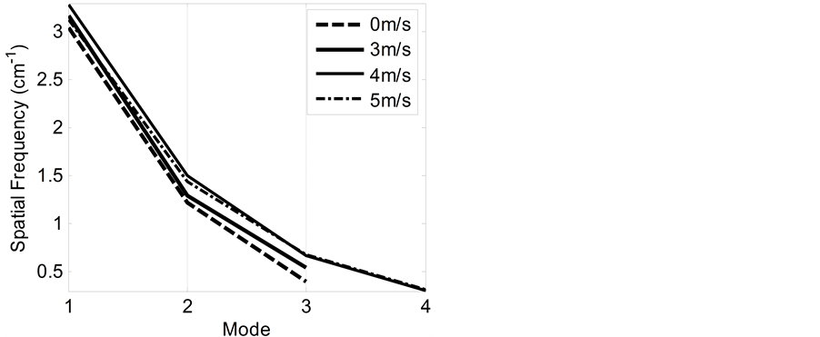
Figure 3. The distribution of the mean spatial frequencies along the empirical modes for different wind speeds.
and 4 m/s reach 0.1210 cm−1 and 0.2664 cm−1 separately. These can be understood as the decreasing of length variation for the surface temperature along the wind speed. As for the amplitudes, it follows from Figure 4 that the existence of wind may results in fold increasing of their values. For the case of 5 m/s, the increments of its frequencies decrease slightly relative to that of 4 m/s in the higher parts and increase slightly in the lower parts. Yet those of its amplitudes vary in the inverse manner.
5. Distributions for Temporal Frequency and Amplitude
In addition to the spatial variation of the surface temperature, there is also a temporal one. To make the investigation it requires a synthetic processing on the infrared photographs. Since only 60 ones obtained in each experiment, the extracted time series merely includes 60 points which can not afford an enough decomposition by the ESMD method. Notice that the temperature of every two adjacent pixels almost vary in the similar manner, to reflect the temporal variation of surface temperature in statistic sense, we prolong the time series to 600 points with adding that of 10 adjacent pixels in turn. We have checked the decomposition results for the cases of 60 and 600 points. Their temporal frequency and amplitude almost accord with each other. To make the statistic result more objective, we compose 5 prolonged time series in a random way and use their average value to reflect the temperature variation for each case. For example, for the no-wind case we have chosen the pixels between 1 - 10, 51 - 60, 101 - 110, 151 - 160 and 201 - 210 separately. At this time, the final results are given in Figure 5 and Figure 6. They indicate that, on the whole, the existence of wind may increase the temporal frequencies and amplitudes of almost all the modes (represent different time scales). The adding of the wind speed, particularly from 4 m/s to 5 m/s, may decrease the variation of surface temperature, not only for the frequency but also for the amplitude. This result accords with that in [6] and it implies a enhanced mixing and a weakened temperature gradient. In addition, Figure 5 also shows an interesting phenomenon that the highest frequency of the
6. Summary
The infrared photographs at the air-water interface of a tank under different wind speeds have been analyzed. With the help of ESMD method, the stochastic temperature sequences are decomposed into several empirical modes of general periodic forms which are very conductive to change analysis. As the spatial sequences concerned, the statistic results indicate that, within certain limits (<5 m/s), as the wind speed increases the spatial frequencies at different scales increase along in a certain extent. Specifically speaking, relative to the no-wind case which has three modes with mean frequencies 3.0401 cm−1, 1.2182 cm−1 and 0.3993 cm−1, respectively, the
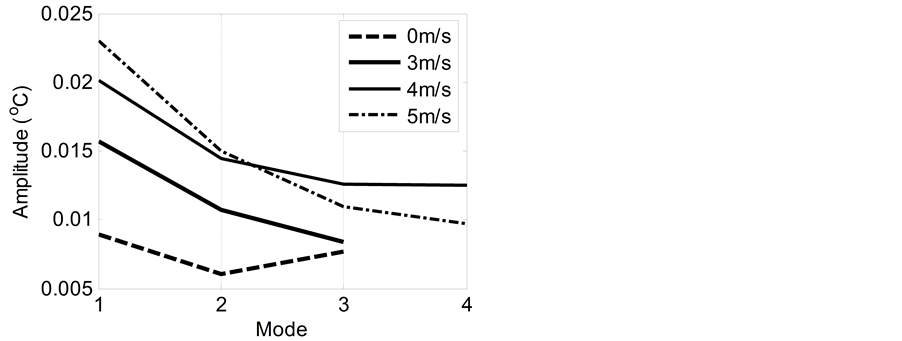
Figure 4. The distribution of the mean spatial amplitudes along the empirical modes for different wind speeds.
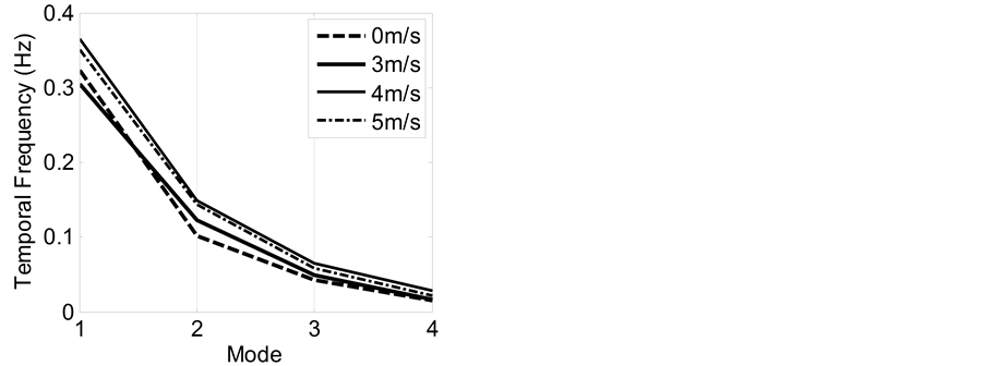
Figure 5. The distribution of the mean temporal frequencies along the empirical modes for different wind speeds.
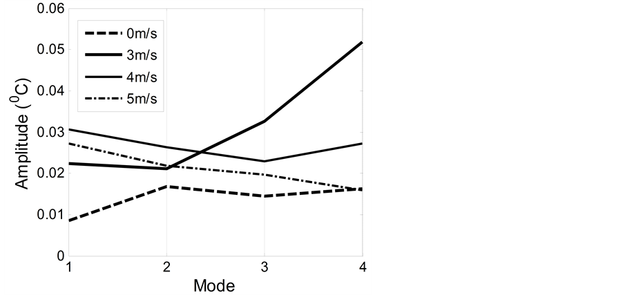
Figure 6. The distribution of the mean temporal amplitudes along the empirical modes for different wind speeds.
mean increments of those for 3 m/s and 4 m/s reach 0.1210 cm−1 and 0.2664 cm−1, respectively. As for the amplitudes, the existence of wind may result in fold increasing of their values. The analysis on the temporal sequences not only reveals the same thing as above but also indicates that when the wind speed is added from 4 m/s to 5 m/s both frequency and amplitude of the surface temperature decrease. This result accords with that given by Veron et al. in 2008 which can be understood as an enhanced mixing and a weakened temperature gradient under the force of wind blowing. In all, the data analyses on the tank experiments indicate that, within certain limits, both spatial and temporal frequencies of the surface temperature increase along the wind speed. As for the amplitudes, the existence of wind may results in fold increasing of their values. For a too high wind speed, the decreasing tendency appears for the frequency and amplitude.
Acknowledgements
We thank the supports from: 1) Fund of Oceanic Telemetry Engineering and Technology Research Center, State Oceanic Administration (No.2013005); 2) the National Natural Science Fund of China (No.41376030); 3) the Shandong Province Natural Science Fund (No. ZR2012 DM004). The experiment data are offered by Dr. Zhaohui Han, here we also express our thanks for his help.
References
- Wang, J.L. and Li, Z.J. (2013) Extreme-Point Symmetric Mode Decomposition Method for Data Processing. Advances in Adaptive Data Analysis, 5, Article ID: 1350015. http://dx.doi.org/10.1142/S1793536913500155
- Wang, J.L. and Li, Z.J. (2015) Extreme-Point Symmetric Mode Decomposition Method: A New Approach for Data Analysis and Scientific Exploration. Beijing. China Higher Education Press, Beijing.
- Huang, N.E., Shen, Z., Long, S.R., et al. (1998) The Empirical Mode Decomposition and the Hilbert Spectrum for Nonlinear and Non-Stationary Time Series Analysis. Proceedings of the Royal Society of London, Series A, 454, 903- 995. http://dx.doi.org/10.1098/rspa.1998.0193
- Wang, J.L. and Li, Z.J. (2014) The ESMD Method for Climate Data Analysis. Climate Change Research Letters, 3, 1-5. http://dx.doi.org/10.12677/CCRL.2014.31001
- Li, H.F., Wang, J.L. and Li, Z.J. (2013) Application of ESMD Method to Air-Sea Flux Investigation. International Journal of Geosciences, 4, 8-11. http://dx.doi.org/10.4236/ijg.2013.45B002
- Veron, F., Melville, W.K. and Lenain, L. (2008) Infrared Techniques for Measuring Ocean Surface Processes. Journal of Atmospheric and Oceanic Technology, 25, 307-326. http://dx.doi.org/10.1175/2007JTECHO524.1
- Mueller, J.A. and Veron, F. (2010) Bulk Formulation of the Heat and Water Vapor Flues at the Air-Sea Interface including Nonmolecular Contributions. Journal of the Atmospheric Sciences, 67, 234-247. http://dx.doi.org/10.1175/2009JAS3061.1
- Han, Z.H. (2013) Research on the Lab Infrared Observational Method for Air-Sea Heat Flux. The Master’s Thesis for Qingdao University, Qingdao.