International Journal of Geosciences
Vol.5 No.8(2014), Article ID:48315,14 pages
DOI:10.4236/ijg.2014.58070
Tracing of the Avenue of the Ram-Headed Sphinxes Remains Using Geophysical Investigations, Luxor, Egypt
Alhussein A. Basheer*, Abdelnasser M. Abdel-motaal, Ahmed El-Kotb, Ayman I. Taha, Mohammed A. Abdalla
National Research Institute of Astronomy and Geophysics (NRIAG), Cairo, Egypt
Email: *Alhussein.adham.basheer.mohammed@gmail.com
Copyright © 2014 by authors and Scientific Research Publishing Inc.
This work is licensed under the Creative Commons Attribution International License (CC BY).
http://creativecommons.org/licenses/by/4.0/
![]()
![]()

Received 10 March 2014; revised 8 April 2014, accepted 2 May 2014
ABSTRACT
Throughout 3000 years ago, over the New Kingdom in the Pharaonic period, the Ram-headed Sphinxes Avenue connected Karnak and the Temples of Luxor, a processional avenue was lined on both sides by 1200 statues of sphinxes. The lining of the avenue was erased. Centuries over centuries this avenue has been buried with its statues under about 2 m of silt and sand, and urban development covered it with housing, asphaltic streets, and other structures, obscuring its route and interrupting this dramatic connection. This paper focuses on the discovery of some of these Sphinx statuses and remains at a suggested part of the avenue using both near-surface magnetic and shallow seismic refraction methods. A gradiometer survey was conducted in an area that amounted 576 m2 as (48 m × 12 m) to measure the vertical magnetic gradient with a high resolution instrument with 0.25 m sampling interval. A superior detection was accomplished by using the analytic signal and Euler deconvolution techniques. The shallow seismic refraction survey was done in the same area to illustrate the lithology of layers material with 1 m interval; both P and S waves were measured to calculate the geotechnical properties of the area to sustain the sketch of structures’ boundaries. We have lucratively detected six main structures; they can be the pedestal of these Ram-headed Sphinx statues. Mining a small part of the study area has proven the reliability of, both the magnetic and shallow seismic refraction discoveries, and the shallowness and composition of the detected features.
Keywords:The Avenue of the Ram-Headed Sphinxes Remains, Near-Surface Magnetic Profiling, Shallow Seismic Refraction Investigation, Luxor, Egypt
1. Introduction
Luxor is considered as the home of world-renowned monuments. Karnak Temple (the most impressive Pharaonic temple in Egypt) and Luxor Temple represent some of the finest examples of mankind’s early civilization. They are ranked as some of the greatest cultural achievements.
During the Pharaonic time, the Avenue of the Sphinxes connected between the Temples of Luxor and Karnak, a processional avenue was lined on both sides by 1200 statues of sphinxes. The government of Luxor has a new orientation to renovate this avenue along the 2.4 kilometer length to improve the tourism, increase the vitality of the city center, and make the city look like an open museum.
In the present study, we tried to apply two famous geophysics tools in archaeological discovery, which are near-surface magnetic survey and shallow seismic refraction survey, to help in detecting the remains of these sphinxes. This study will help in verifying its location and underlining its archaeological potential.
The chosen study area near asphalted road covers an area of about 567 m2. It is portrayed between latitudes 25˚42'35.24" and 25˚42'36.63"N and longitudes 32˚39'1.09" and 32˚39'2.61"E (Figure 1).
2. Data Acquesition
2.1. Near-Surface Magnetic Survey
The study area was cleaned from any visible iron materials in the surface. The corners of the surveyed area of 12 m × 48 m (576 m2) are marked with wooden sticks. The study area is divided into 18 grids; each grid was set to 4 × 8 m (Figure 2). The distances and traverses were measured and detected using non-magnetic tapes and ropes. The ropes are marked at 0.25 m interval. The internal corners of each grid are marked by small plastic sticks.
The fluxgate gradiometer (FM36 from Geoscan Research (1987) [1] with 0.5 m sensor spacing) was correctly balanced and nulled over an area of uniform local magnetic field. This procedure was repeated after the end of each two grids survey. The gradiometer sensitivity was set to 0.1 nT. The measurements of the vertical magnetic gradient have been taken through successive parallel traverses separated by 0.25 m interval. The readings were then logged every 0.25 m and downloaded to a notebook computer in the field. The total number of the readings acquired over the study area is 9216. They were collected and stored in the FM36 memory. The topography surface was almost flat, which is favored in the gradiometer survey.
2.2. Seismic Survey
Seismic exploration involves generation of seismic waves and recording the arrival times of these waves from
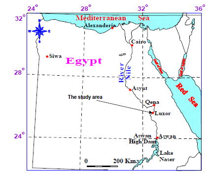
Figure 1. General location map of the study area.
the source to the series of geophones [2] . Seismic refraction method is the most widely applied as a reconnaissance tool in newly-explored areas, especially in archaeological projects. It is mostly used in the mapping of the layers at shallow depth; moreover, layer thicknesses and some data about lithology can be obtained. Seismic refraction is used to evaluate the necessary parameters for structures, or to illustrate the different lithological subsurfaces layers, and the environmental conditions that overcome in the site.
The survey has been accomplished using 48 channels signal enhancement seismograph “GEOMETRICS SMARTSEIS” for every profile. Every profile has 48 m length as 1 m between every geophone (Figure 2). (EST-20DG) geophone type has been used, these geophones are recognized by dual rotating coil structure, key contactor plated silver, high spurious frequency, Wide band, lower distortion that is smaller than 0.1%, main parameters that are controlled within ±2.5%, high signal to noise, small phase difference, and high dynamic resolution.
The vibration generator has been used to generate P and S waves; this source is switched to provide the time break to the seismograph. The power of the vibration generator helps in avoiding the loosing of waves strength that may be caused by “blind layer” in some conditions.
The low pass filter in the recording system has 7 - 10 MHz as a frequency response, which is suitable for the recording condition, and is positioned before the analog-digital conversion circuit. Some special arrangement has done to create and detect un-noisy SH-wave in the field (Figure 3). The first step was to switch the vibration generator to SH-wave position “To pulse in 45˚ angle” in the shot point position. The second step was to make a hole between the first geophone and the shot point; this hole makes the P-waves, which will be certainly created with SH-waves, deploying in very high distributed material “air”.
P-waves will be delayed and weakened, so the most waves that reach geophones will be the SH-waves and geophones can only detect the SH-wave. On the other hand, the SH-waves are less in values than P-waves, so it can be digitally separated by software program. The shallow seismic survey was conducted in 2 days (20 hours) to present twenty four seismic general-profiles covered the spot area.
Satellite image of the study area
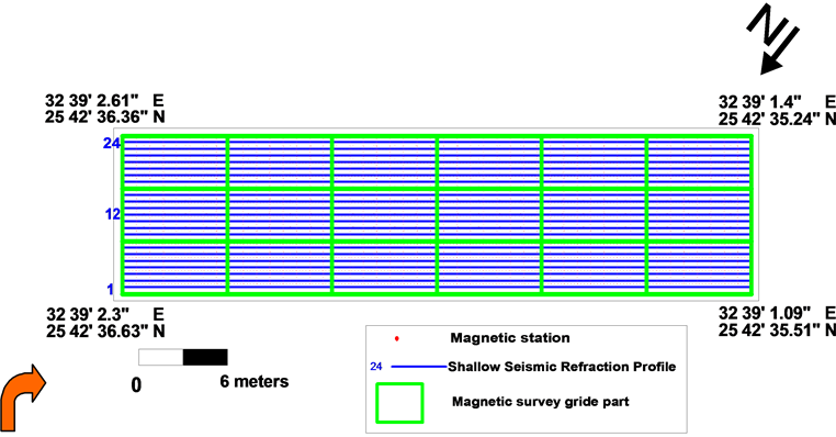
Figure 2. Location map of the study area shows near-surface magnetic stations, magnetic grid lines and SSR profiles.
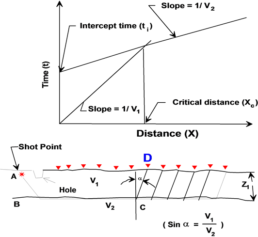
Figure 3. Velocity estimation by using the slope method calculation with shot point and geophones array in field [3] .
3. Data Interpretation
3.1. Near-Surface Magnetic Data Interpretation and Discussion
Untreated magnetic data of Figure 4 display magnetic effects from many sources. Apart from the visible blocks anomaly in the middle part of the image, these anomalies are larger than expected sources due to undesirable field defects and other noise sources.
According to historical references, the near features, and the extension of the sphinxes avenue near the study area, we observed that:
a) The measurements of the vertical magnetic gradient were conducted using 0.25 m parallel traverses at 0.25 m sampling interval.
b) The obtained Shade-plot of the raw magnetic data ranges from −160.00 to160.00 nT/m (Figure 4).
c) Some archaeological parts are clearly present in the form of tables with anomalies’ strengths ranging from −1 to −30 nT/m.
d) Gradiometer data are bipolar and the archaeological signature isn’t under −30 nT/m, so we clipped the data at ±30 nT/m to reduce spike effects from the hidden ferrous objects (Figure 5).
During the analysis, the following steps were carried out:
1) We removed edge discontinuities between grids that were arisen by subtracting the mean of each sub-grid, employing the readings below a threshold of 0.25 of the standard deviation. It’s known that the effects occur due to incorrect zeroing or zero drift, but the mean of a gradient data set should be zero. This yielded a much improved data set.
2) We smoothed the data that were performed using a Gaussian low-pass filter; thus, enhancing the large weak features that exist in the west part of the study area. The low-pass filter, with reading window size 2, produced the best results and showed clearly the large elongated anomalies. Low-pass filtering emphasized also larger weak archaeological features. It is worth noting that the standard derivations after data processing decreased from −1 nT/m (Figure 5) to 1 nT/m (Figure 6), indicating much reduced errors with illustration of broader and reflecting more archaeological features and less iron spike.
3) Automated techniques of the analytic signal [4] and 3D Euler deconvolution [5] were used to further investigate the above structures (Figure 7 and Figure 8). For example, depths can be either estimated from the shape of the amplitude of the analytic signal [6] or based on the ratio of the analytic signal to its higher derivatives [7] -[9] .
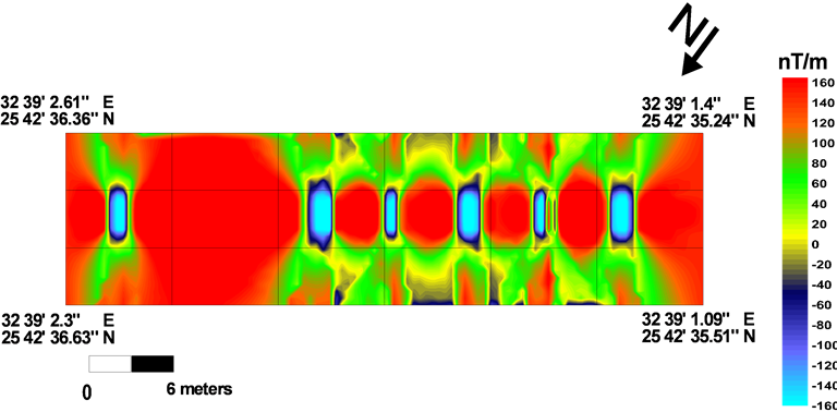
Figure 4. Raw magnetic data.
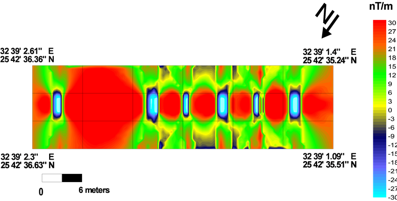
Figure 5. Gradiometer data after removing grid discontinuities, slope error, traverse stripping effect, and removing the iron spikes.
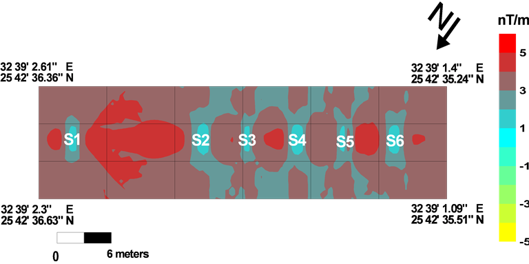
Figure 6. Gradiometer data after applying low-pass filter and interpolation functions.
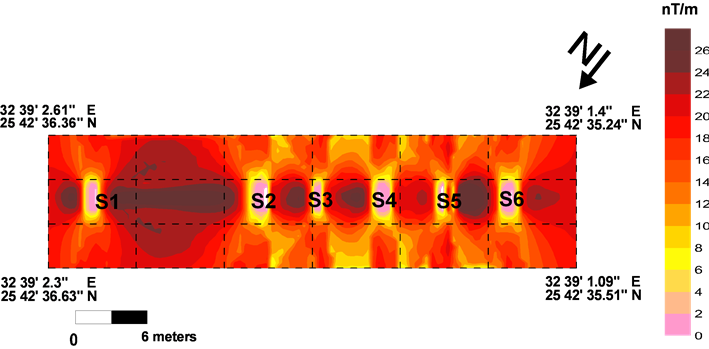
Figure 7. Application of the analytical signal method to the gradiometer data.

Figure 8. Application of depth estimation after the application of 3D Euler deconvolution.
In the present work, we applied the higher derivatives approach of the analytic signal [10] for the detection of archaeological bodies from magnetic data.
Accordingly, the horizontal locations of the magnetic discoveries can be estimated by the maxima of the amplitude of the analytic signal (An).
Following Debeglia and Corpel (1997) [11] , the amplitude of the nth order derivative analytic signal An (x, y) can be expressed in terms of the vertical or the horizontal derivative of M as:
 (1)
(1)
where the superscript z denotes the vertical derivative of the field.
The An (x, y) and its higher order derivatives can be easily computed in a number of ways.
Salem and Ravat (2003) [10] combined application of the analytic signal and Euler method, so the depth of archaeological bodies can be estimated by:
 (2)
(2)
where |A1| and |A2| are the amplitudes of the analytic signal of the vertical gradient anomaly and its first-order derivative.
 (3)
(3)
we mainly used the analytic signal method after upward continuation to a distance of 0.5 m to enhance the signal-to-noise ratio of the magnetic anomalies (Figure 7).
It is clearly observed that the anomalies produced from application of the analytical signal filter may be located in places of archaeological bodies. These bodies look like the remains of sphinxes bases. Five of them (S2, S3, S4, S5, S6) are layout in liner direction with stable diameters and stable distances that separate each one of them, with missed one noted between S1 and S2 anomalies. This missing may be due to erosions. By the application of the analytical signal measuring at each anomaly, we can easily calculate its diameters.
3D Euler deconvolution method calculates the depth of these archaeological bodies (Figure 8). The main view shows that these bodies are in form of bases as oblong shapes. These oblongs lie in depth of 5.50 m and have different thicknesses that ranges from 1.75 m as in S4 and S3 to 0.15 m as in S6.
3.2. SSR Data Interpretation and Discussion
The data has been treated using a computer program called SEIPEEDIT [12] to construct the travel time curve, in which the time of the first arrival is plotted versus the geophone offset distance. The time of the first arrival and its velocity are functions of the depth of the refracted interface according to the equation
 (4)
(4)
where V is the velocity, D is the offset distance (the distance between shot point and the detected geophone), and T is the time that wave takes from shot point to geophone. The layer’s parameters (thickness, depths, and the different velocities under each geophone) have been estimated and used to construct geoseismic cross sections (Figure 3).
Seismic velocity in a geologic material is related to the low-strain dynamic modulus of the material. Soil modulus is influenced by density, confinement and cementation. Consequently, P-waves of the seismic velocity in a soil mass are influenced by density, confinement and cementation. Relationships between density, overburden pressure and modulus in cohesionless sands, dust, clay, and limestone have been studied and refined since at least the 1960’s. One of the older relationships [13] that results in velocity change of cohesionless soil with depth, is based on changes in soil modulus that scale to the square root of the effective stress at a given soil density. These results are presented in Figures 12-16. The interpreted vertical velocity gradient presented in these figures is matched very closely with that cohesionless soil relationship. Cohesionless material modulus manifested as seismic velocity is significantly controlled by the effective stress manifested as overburden pressure at subsurface depth. Soil losing is lessening material strength, and thus modulus decreased. This decreased modulus is at least partly independent of overburden pressure and subsurface depth. At shallow depths with relatively little-overburden pressure, loose soil and variability can result in lower seismic velocities than that would occur without variability. Seismic velocity at shallow depths can thus become an interpretation for the presence of variability and cementation [14] .
The inspection of the constructed seismic cross sections could lead to the same result similar to the near-surface magnetic investigation (NSM) results.
We can note that only five profiles (number 11, 12, 13, 14, and 15) show different changes in its velocities, Figure 9 shows time-distance curve of profile no. 13 as a model for them; and the other profiles has not any obvious change in its currently waves, Figure 10 illustrates time-distance curve of profile no. 1 as example for them.
3D maps over the study area have been done; these maps are created out by applying the data of (Perpendicular waves, shear waves, Poisson’s ratio, The Standard Penetration Test (SPT) as N-value, and allowable bearing capacity “Qa”) on the places of geophones positions. We chose these geotechnical properties to indicate and figure the natural of undersurface bodies. The chosen depths in these maps depended on the cross-sections of profiles, suggested thickness of bodies appear on it, and the results of 3D Euler magnetic map.
The distribution of P-waves is shown in Figure 11, ranges between 430.18 m/sec. to 444.33 m/sec. in surface layer to 3.75 m depth. By increasing depth, velocity reaches about 753 m/sec. in six sites. This change appears as two features in the eastern part of the study area at depth 3.75 m, and as three features at depth 4.75, and six
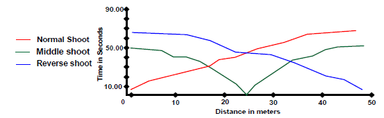
Figure 9. Travel Time-Distance curve along profile 13.
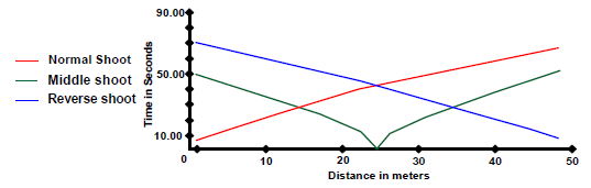
Figure 10. Travel Time-Distance curve along profile 1.
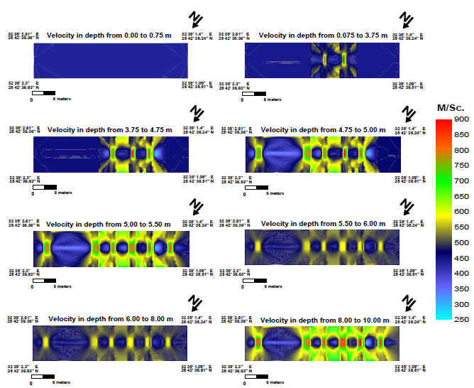
Figure 11. 3D-map of P-Velocity on the study area.
features at depth 5.5 m. The effects of these bodies were continuous with the depth but with obvious decreases in values.
The allocation of S-waves is illustrated in Figure 12, ranges between 275.6 m/sec. to 477.3 m/sec. in surface layer to 3.75 m depth. By increasing in depth, velocity reaches about 285 m/sec. in six sites. This vary appears as two features in the eastern part of the study area at depth 3.75 m, and as three features at depth 4.75, and six features at depth 5.5 m. The influence of these bodies was unremitting by depth but with obvious decreases in values.
The Poisson’s Ratio is defined as “the ration of the fractional transverse construction to the fractional longitudinal extension” [15] . We can calculate Poisson’s Ratio by equation:
 (5)
(5)
The same effect of the presence of these bodies appears in Figure 13, ratio ranges from 0.1505 to 0.151 but it changes to about 0.267 in the sites of these bodies.
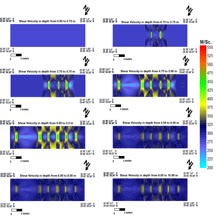
Figure 12. 3D-map of SH-Velocity on the study area.
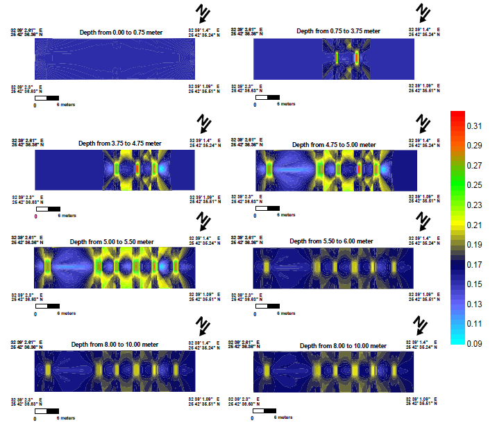
Figure 13. 3D-map of Poisson’s ratio on the study area.
Figure 14 shows the distribution of the Standard Penetration Test (SPT) in the study area. This test is geotechnical known as “the resistance to penetration by normalized cylindrical bars under standard load”. The Standard Penetration Test (SPT) can be estimated from velocity of S-waves by equation:
 (6)
(6)
We refer to it as N-Value, which ranges between to 27.5 to 37.77 over the area with accepted change to about 102.5 in these bodies’ sites.
The allowable bearing capacity is the maximum load to be considerable to avoid shear failure or sand liquefaction; it can be termed as allowable bearing pressure too, and we refer to it as Qa. It can be easily calculated by [16] equation:
![]() (7)
(7)
Figure 15 shows the allotment of Qa in the study area. The values vary from 13.7 to 28.5 K.Pa, change appears in the same bodies’ sites to reach about 53.6 K.Pa.
From these maps, it is clearly obvious that there are six bodies (S1, S2, S3, S4, S5, and S6) with different lithology and density. These bodies may consist of sandstone rock with difference in lithology from the clay and surrounding mud. Its thicknesses vary from 1.75 m to 0.15 m and have depths between 3.75 m and 5.5 m.
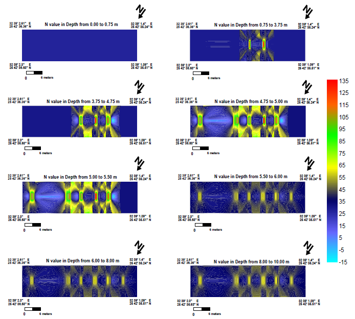
Figure 14. 3D-map of N-value on the study area.
4. Conclusions
The present study has been mainly conducted to detect the site of the avenue of sphinxes remains in old Luxor city. The study involves carrying out two main geophysical integrated techniques; the first technique embraces executing near-surface magnetic survey. The study area is split to 18 grids, and every grid has an area as 4 × 8 m using FM36 system and reading 9216 points.
The second technique of the study depends on the analysis of the seismic refraction data acquired using twenty four shallow seismic refraction profiles distributed over the study area. Through the NSM survey, the penetrated depth reached about 7 m while the penetrated depth reached with the SSR varied from 9.2 m under geophone No. 12 of profile 3 to 10.33 m under geophone 21 of profile 22. The difference in detection of boundaries and edges between magnetic survey and seismic survey may be due to the interval between the measured places on each method, which is close in near-surface magnetic survey (0.5 m) and relatively wide in shallow seismic refraction survey (0.5 m between profiles, and 1 m between geophones). This interval is noticeable between profile 10 and 11 in seismic survey, where archaeological body is absent under profile 10 and present in magnetic survey map at 0.25 m in profile 11.
Figure 16 shows the final interpreted shapes, thicknesses, and depth of the detected bodies from both magnetic and shallow seismic refraction methods.
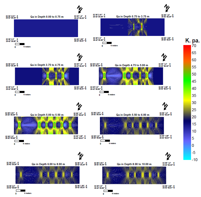
Figure 15. 3D-map of Qa on the study area.
The integrated results obtained from the interpretation of both of the NSM and the SSR records were conducted over the suspected site in the study area are as follows:
a) Six bodies with oblong shapes appear, and these bodies may be the base of the ram-head sphinx status.
b) These bodies have geometrical shapes, and each base of them has about 2.25 to 2.30 m length and its width about 1.25 m. The distance between each base is about 4 m.
c) These bodies have thicknesses which range from 0.10 to 1.25 m d) These bodies set in depth between 3.75 m and 5.5 m.
e) Missed body can be obvious in the emptiness of the distance between S1 and S2, which may be due to erosion.
f) According to the lateral distribution of the lithological layers’ parameters from both magnetic and shallow seismic refraction surveys, the lithology of these bodies may consist of sandstone rock; this lithology differs from the surrounds area which consists of mud and clay.
Finally, the present study indicates that the discovered archaeological features are at very shallow depths of
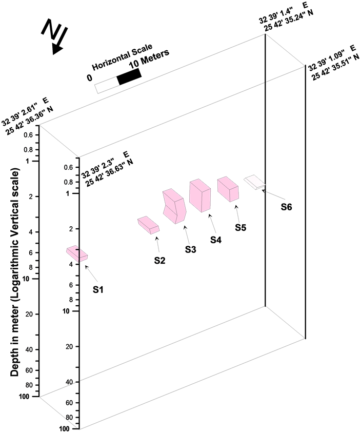
Figure 16. The final interpreted from both magnetic and shallow seismic refraction methods.
less than 2.0 to 10.0 m. Based on these results, we believe that the whole region needs more cooperation between archaeologists and geophysicists to explore its mysterious ancient history more effectively.
References
- Geoscan Research (1987) Instruction Manual Version 1.0 (Fluxgate Gradiometer FM9, FM18, FM36). Geoscan Research, Bradford.
- Dobrin, M.B. (1976) Introduction to Geophysical Prospecting. 3rd Edition, McGraw Hill, New York, 25-56, 292-336, 568-620.
- Basheer, A.A. (2003) Application of Geophysical Techniques at New Qena City. M.Sc. Thesis, Qena Faculty of Science, South Valley University, Qena.
- Nabighian, M.N. (1972) The Analytic Signal of Two-Dimensional Magnetic Bodies with Polygonal Cross-Section: Its Properties and Use for Automated Anomaly Interpretation. Geophysics, 37, 507-517.http://dx.doi.org/10.1190/1.1440276
- Reid, A.B., Allsop, J.M., Granser, H., Millet, A.J. and Somerton, I.W. (1990) Magnetic Interpretation in Three Dimensions Using Euler Deconvolution. Geophysics, 55, 80-91. http://dx.doi.org/10.1190/1.1442774
- Roest, W.R., Verhoef, J. and Pilkington, M. (1992) Magnetic Interpretation Using 3-D Analytic Signal. Geophysics, 57, 116-125. http://dx.doi.org/10.1190/1.1443174
- Hsu, S.K., Sibuet, J.C. and Shyu, C.T. (1996) High-Resolution Detection of Geologic Boundaries from Potential Anomalies: An Enhanced Analytic Signal Technique. Geophysics, 61, 373-386. http://dx.doi.org/10.1190/1.1443966
- Bastani, M. and Pedersen, L.B. (2001) Automatic Interpretation of Magnetic Dikes Parameters Using the Analytic Signal Technique. Geophysics, 66, 551-561. http://dx.doi.org/10.1190/1.1444946
- Salem, A., Ravat, D., Gamey, T.J. and Ushijima, K. (2002) Analytic Signal Approach and Its Applicability in Environmental Magnetic Investigations. Journal of Applied Geophysics, 49, 231-244. http://dx.doi.org/10.1016/S0926-9851(02)00125-8
- Salem, A. and Ravat, D. (2003) A Combined Analytic Signal and Euler Method (AN EUL) for Automatic Interpretation of Magnetic Data. Geophysics, 68, 1952-1961. http://dx.doi.org/10.1190/1.1635049
- Debeglia, N. and Corpel, J. (1997) Automatic 3-D Interpretation of Potential Field Data Using Analytic Signal Derivatives. Geophysics, 62, 87-96. http://dx.doi.org/10.1190/1.1444149
- SEIPEEDIT Program Version 6.23 (2002) Seismic Interpretation Program Software. OYO Company, New York. www.OYO.com
- Richart, F.E., Hall, J.R. and Woods, R.D. (1970) Vibrations of Soils and Foundations. Prentice-Hall Inc., Upper Saddle River.
- Rucker, M.L. (2000) Applying the Seismic Refraction Technique to Exploration for Transportation Facilities, in Geophysics 2000. The First International Conference on the Application of Geophysical Methodologies to Transportation Facilities and Infrastructure, St. Louis, 11-15 December 2000, 1-3.
- Sheriff, R.E. (1991) Encyclopedic Dictionary of Exploration Geophysics. 3rd Edition, Society of Exploration Geophysicists, 89-94.
- Abd El-Rahman, et al. (1991) Rock Material Competence Assassed by Seismic Measurements with Emphasis on Soil Competence Scales and Their Applications in Some Urban Areas in Yemen, EGS. Proceedings of the 9th Annual Meeting, 9, 205-230.
NOTES

*Corresponding author.