International Journal of Geosciences
Vol. 4 No. 3 (2013) , Article ID: 31453 , 9 pages DOI:10.4236/ijg.2013.43050
Stress and Strain Accumulation Due to a Long Dip-Slip Fault Movement in an Elastic-Layer over a Viscoelastic Half Space Model of the Lithosphere-Asthenosphere System
1Department of Applied Mathematics, University of Calcutta, Kolkata, India
2Department of Basic Science and Humanities, Meghnad Saha Institute of Technology (A Unit of Techno India Group), Kolkata, India
Email: dr.sanjaysen@rediff.com, skd.sxccal@gmail.com
Copyright © 2013 Sanjay Sen, Subrata Kr. Debnath. This is an open access article distributed under the Creative Commons Attribution License, which permits unrestricted use, distribution, and reproduction in any medium, provided the original work is properly cited.
Received January 12, 2013; revised February 14, 2013; accepted March 12, 2013
Keywords: Aseismic Period; Dip-Slip Fault; Earthquake Prediction; Mantle Convection; Plate Movements; Stress Accumulation; Tectonic Process; Viscoelastic-Layered Model
ABSTRACT
Most of the earthquake faults in North-East India, China, mid Atlantic-ridge, the Pacific seismic belt and Japan are found to be predominantly dip-slip in nature. In the present paper a dip-slip fault is taken situated in an elastic layer over a viscoelastic half space representing the lithosphere-asthenosphere system. A movement of the dip-slip nature across the fault occurs when the accumulated stress due to various tectonic reasons e.g. mantle convection etc., exceeds the local friction and cohesive forces across the fault. The movement is assumed to be slipping in nature, expressions for displacements, stresses and strains are obtained by solving associated boundary value problem with the help of integral transformation and Green’s function method and a suitable numerical methods is used for computation. A detailed study of these expressions may give some ideas about the nature of stress accumulation in the system, which in turn will be helpful in formulating an earthquake prediction programme.
1. Introduction
It is the observational fact that while some faults are strike slip (finite or infinite in length) in nature, there are faults (e.g., Sierra Nevada/Owens valley: Basin and Range faults, Rocky Mountains, Himalayas, Atlantic fault of central Greece—a steeply dipping fault with dip 60, 80 (deg)) where the surface level changes during the motion i.e. the faults are dip-slip in nature.
A pioneering work involving static ground deformation in elastic media was initiated by [1,2]. Ref. [3] did a wonderful work in analyzing the displacement, stress and strain for dip-slip movement. Later some theoretical models in this direction have been formulated by a number of authors like [4-30]. Ref. [31] has discussed various aspects of fault movement in his book. Ref. [32] has discussed stress accumulation near buried fault in lithosphere-asthenosphere system. The work of [33] can also be mentioned in these connections.
In most of these works the medium were taken to be elastic and/or viscoelastic, but a layered model with elastic layer(s) over elastic or viscoelastic half space will be a more realistic one for lithosphere-asthenosphere system.
In the present case we consider a long dip-slip fault situated in an elastic layer over a viscoelastic half space which reaches up to the free surface. The medium is under the influence of tectonic forces due to mantle convection or some related phenomena. The fault is assumed to undergo a slipping movement when the stresses in the region exceed certain threshold values.
In our paper, we consider an elastic layer over a viscoelastic half space to represent the lithosphere-asthenosphere system, with constant rigidity (2.0 ´ 105 Mpa) and viscosity (1020 - 1021 pa∙s) following the observational data mentioned by [34,35]. Analytical expressions for displacements, stresses and strains in the system are obtained both before and after the fault movement using appropriate mathematical technique involving integral transformation and Green’s function. Numerical computational works have been carried out with suitable values of the model parameters and the nature of the stress and strain accumulation in the medium have been investigated.
2. Formulation
We consider a long dip-slip fault F and width D situated in an elastic layer over a viscoelastic half space of linear Maxwell type.
A Cartesian co-ordinate system is used with a suitable point O on the strike of the fault as the originY1 axis along the strike of the fault, Y2 axis is as shown in Figure 1 and y3 axis pointing downwards. We choose another co ordinate system ,
,  and
and  axes as shown in Figure 1 below, so that the fault is given by
 . Let q be the dip of the fault F and v1, w1 be the displacement components along y2 and y3 axes respectively for the layer and v2, w2 be that for the half-space.
 , are stress and strain, k = 1 for the layer and k = 2 for the half-space and i, j = 2, 3.

Figure 1. Section of the model by the plane y1 = 0.
2.1. For an Elastic Medium the Constitutive Equations Are Taken as
For the layer: M1
 (2.1)
(2.1)
 (2.2)
(2.2)
 (2.3)
(2.3)
2.2. For a Viscoelastic Maxwell Type Medium the Constitutive Equations Are Taken as
For half-space: M2
 (2.4)
(2.4)
 (2.5)
(2.5)
 (2.6)
(2.6)
where, μ1, μ2 are the effective rigidity of the layer and the half-space respectively and h2 is the effective viscosity of the half-space.
2.3. The Stresses Satisfy the Following Equations (Assuming No Changes in the External Body Force)
For M1:
 (2.7)
(2.7)
 (2.8)
(2.8)
where 
For M2:
 (2.9)
(2.9)
 (2.10)
where  and assuming quasi-static deformation for which the inertia term are neglected.
The boundary conditions are taken as, with t = 0 representing an instant when the medium is aseismic state.
 (2.11)
On the free surface y3 = 0, t > 0
 (2.12)
 (2.13)
Also as y3 →
 (2.14)
 (2.15)
 (2.16)
 (2.17)
[where  is the shear stress maintained by mantle convection and other tectonic phenomena throughout the medium].
2.4. The Initial Conditions Are
Let  and
and  be the value of (v2), (w2),
  and
and  at time t = 0 which are functions of y2, y3 and satisfy the relations (2.1)-(2.17).
a) Solutions in the absence of any fault dislocation [36,37]:
The boundary value problem given by (2.1)-(2.17), can be solved by taking Laplace transformation with respect to time “t” of all the constitutive equations and the boundary conditions. On taking the inverse Laplace transformation we get the solutions for displacement, stresses as:
For M1:

 (A)
(A)
From the above solution we find that  remain unchanged from the initial one, while
  increases linearly with time if we assume that
  to be constant. We assume that the geological conditions as well as the characteristic of the fault is such that when
  reaches some critical value, say
  the fault F undergoes a sudden slip along the dip direction.
The magnitude of the sudden slip shall satisfy the following conditions as discussed by [13].
(C1) Its value will be maximum on the free surface.
(C2) The magnitude of the slip will decrease with y3 as we move downwards and ultimately tends to zero near the lower edge of the fault.
b) Solutions after the fault movements [36,37]:
We assume that after a time T1, the stress component  (which is the main driving force for the dip-slip motion of the fault) exceeds the critical value
 , and the fault F undergoes a sudden slip along the dip direction, characterized by a dislocation across the fault given in (Appendix).
We solve the resulting boundary value problem by modified Green’s function method following [1,2,24] and correspondence principle (as shown in Appendix) and get the solution for displacements, stresses and strain as:
For M1:
or, 
where,
and

and
where,
where,
where,  (B)
(B)
3. Numerical Computations
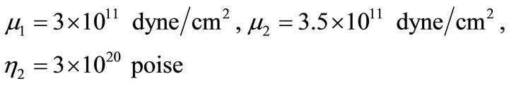
Following [38] and recent studies on rheological behavior of crust and upper mantle by [34,35] the values of the model parameters are taken as:
D = Depth of the fault = 10 km [noting that the depth of all major earthquake faults are in between 10 - 15 km].
H = Thickness of the layer = 40 km. say (though the thickness varies from region to region of the Earth).
 .
.
 (200 bars), [post seismic observations reveal that stress released in major earthquake are of the order of 200 bars, in extreme cases it may be 400 bars]
and, 
We take the function , with W = 1 cm/year, satisfying the conditions stated in
 .
.
We now compute the following quantities:
For layer M1:
 (3.1)
(3.1)
 (3.2)
(3.2)
4. Results and Discussions
The parameters involved in the expressions for displacements and stresses have been assigned appropriate values available from observed data through repeated geodetic surveys prior to and after the seismic events in seismically active regions in South and North America and China. Numerical computations are carried out using this observed values of the parameters as discussed in §3.
4.1. Variation of Vertical Component of Displacement Due to Sudden Slip across the Fault after t1 = 1 Year
“Equation (3.1)” gives us the vertical component of displacement at (y2, y3) due to the movement across the fault for different dip angle q and at different time after the fault movement. We take t1 = 1 year. In Figure 2 the graph shows the nature of surface displacement W1 against y2, the distance from the strike of the fault with q = 90 (in deg). It is observed that the displacements are in opposite directions across the strike of the fault. Their magnitudes gradually decrease and tend to zero as we move away from the fault. This is quite expected as the effect of the fault movement gradually dies out with distance. The sudden changes of W1 near y2 = 0 is due to the dip-slip motion along the fault. This is in good conformity with the result shown in Paul Segal (2010). Figure 3 shows the variation of W1 with depth y3 along the vertical through a point y2 = 5 km. for a vertical fault with q = 90 (in deg). It shows that W1 decreases sharply up to a depth of about 18 km. and thereafter diminishes to zero at a slower rate, and continuously decreases to zero for y3 > 100 km.
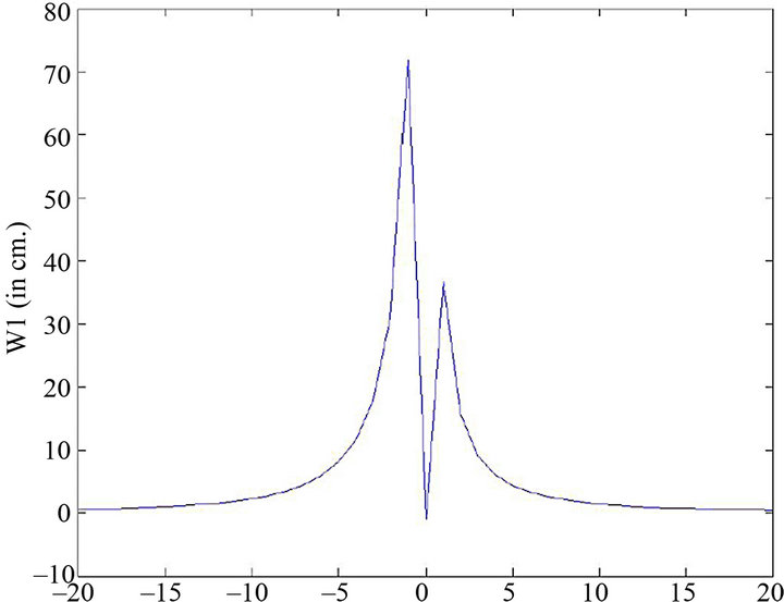
Figure 2. Variation of vertical component of displacement W1 with y2 for y3 = 0 km, q = 90 (deg), t1 = 1 year due to the fault movement.
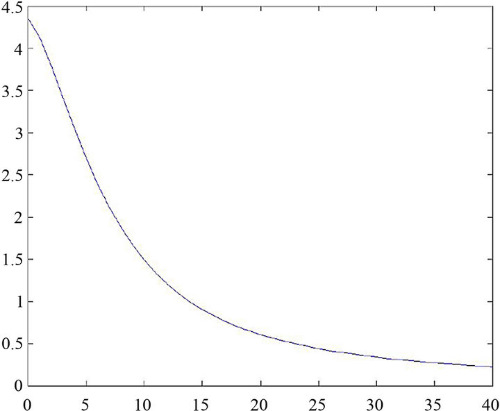
Figure 3. Variation of vertical component of displacement W1 with depth y3 for y2 = 2 km, q = 90 (deg), t1 = 1 year due to the fault movement.
4.2. Variation with Depth of the Main Driving Stress t2(3( in the Dip-Slip Direction Due to the Movement across F
Figures 4-7 show the variation of  with depth y3 for various q and some specific values of y2.
In Figure 4 it is found that for a dip-slip fault with dip angle q = 30 and along the line y2 = 8 km,  undergoes a change (in one year) due to the slip movement across F. Initially there is a very small region of stressrelease just below the free surface (0 < y3 < 4.5 km). Thereafter, the rate of stress-release decreases up to a depth of 13 km and then stress begin to accumulate in the region from y3 = 13 km to y3 = 20 km after that the rate of stress accumulation gradually decreases continuously and becomes negligibly small at a depth of 50 km.
Figure 5 shows the variation of main driving stress component  with the depth of y2 = 8 km, t1 = 1 year
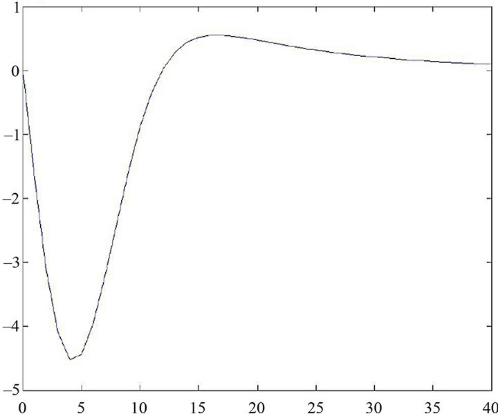
Figure 4. Variation of stress t2¢3¢ with depth y3 for y2 = 8 km, q = 30 (deg), t1 = 1 year due to the fault movement.
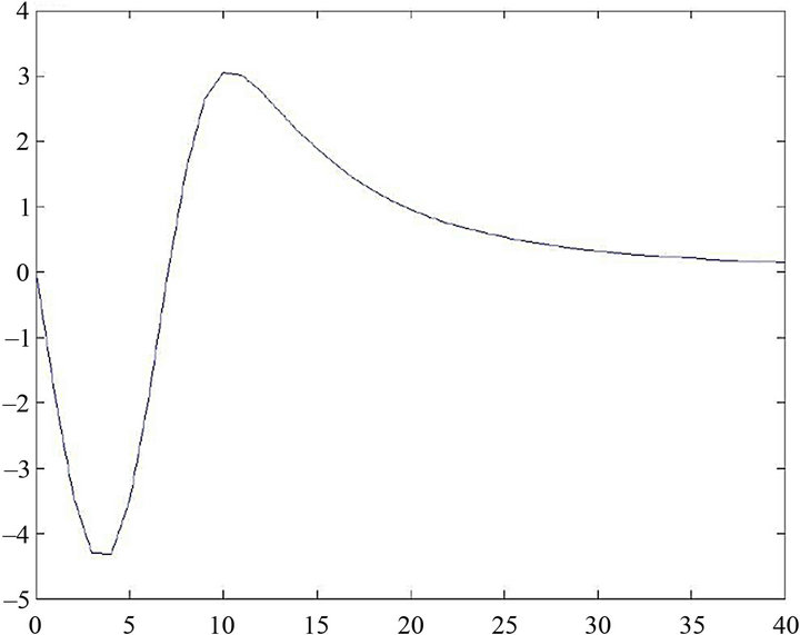
Figure 5. Variation of stress t2¢3¢ with depth y3 for y2 = 8 km, q = 45 (deg), t1 = 1 year due to the fault movement.
due to the slip movement across the fault at a deep angle q = 45 (degree). The rate of stress release increases up to a depth of 4 km. Then the rate decreases up to a depth of about 4 to 8 km. And then begin to accumulate from 8 to 20 km. with a maximum of 3 bar per year at a depth of about 10 km. And continuously decreases to zero at about 75 km from the free surface. Figure 6 shows the variation of stress component  for y2 = 9 km, t1 = 1 year and dip angle q = 60 (degree) with the depth due to the slip across the fault.
We see stress releases in the region 0 ≤ y3 ≤ 40 km. with increasing rate up to y3 = 6.5 km and then with decreasing rate and become 0 at a depth about 100 km.
For vertical dip-slip fault the nature is the same with less numerical values, which is explained by Figure 7.
For vertical dip-slip fault the nature is the same with less numerical values, which is explained by Figure 2.
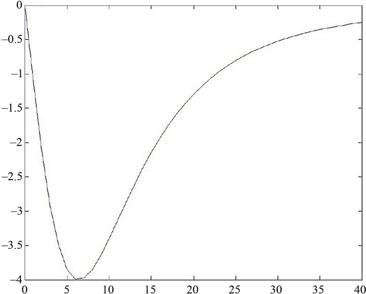
Figure 6. Variation of stress t2¢3¢ with depth y3 for y2 = 9 km, t1 = 1 year, q = 60 (deg) due to fault movement.
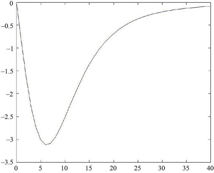
Figure 7. Variation of stress t2¢3¢ with depth y3 for y2 = 10 km, t1 = 1 year, q = 90 (deg) due to fault movement.
5. Conclusions
Thus in the above discussion we see that due to slip movement in the dip-slip fault, there are regions where stress get released and there are certain other regions where stress accumulates. The rate of stress release/accumulation depends essentially on the dip-angle q and the distance y2 from the fault.
If there were a second fault situated in the region where stress get released due to the movement across the first fault, the possibility of a movement across the second fault would likes to be deferred further. On the other hand, if the second fault be situated in the region where stress accumulates, the possibility of a movement across the second fault will be enhanced. The study of such interactions among neighboring faults is very important in seismically active regions where there are a number of neighboring faults exist.
6. Acknowledgements
One of the authors (Subrata Kr. Debnath) thanks the Principal and Head of the Department of Basic Science and Humanities, Meghnad Saha Institute of Technology, a unit of Techno India Group (INDIA), for allowing me to pursue the research, and also thanks the Geological Survey of India, ISI, Kolkata, for providing me the library facilities. Department of Applied Mathematics, University of Calcutta for providing the library facilities.
REFERENCES
- T. Maruyama, “Statical Elastic Dislocations in an Infinite and Semi-Infinite Medium,” Bull Earthquake Research Institute, Tokyo University, Tokyo, 1964.
- T. Maruyama, “On Two Dimensional Dislocations in an Infinite and Semi-Infinite Medium,” Bull Earthquake Research Institute, Tokyo University, Tokyo, 1966.
- J. C. Savage and L. M. Hastie, “Surface Deformation Associated with Dip Slip Faulting,” 1966.
- K. Rybicki, “The Elastic Residual Field of a Very Long Strike Slip Fault in the Presence of a Discontinuity,” Bulletin of the Seismological Society of America, Vol. 61, 1971, pp. 79-92.
- L. Mansinha and D. E. Smyllie, “The Displacement Fields of Inclined Faults,” Bulletin of the Seismological Society of America, Vol. 61, No. 5, 1971, pp. 1433-1440.
- R. Sato, “Stress Drop of Finite Fault,” Journal of Physics of the Earth, Vol. 20, 1972, pp. 397-407.
- S. J. Singh and M. Rosenman, “Quasi Static Deformation of a Viscoelastic Half-Space by a Displacement Dislocation,” Physics of the Earth and Planetary Interiors, Vol. 8, 1974, pp. 87-101.
- A. Nur and G. Mavko, “Post-Seismic Viscoelastic Rebound,” Science, Vol. 183, 1974, pp. 204-206.
- R. Sato and T. Yamashita, “Static Deformations in an Obliquely Layered Medium Part-II Dip-Slip Fault,” Journal of Physics of the Earth, Vol. 23, 1975, pp. 113-125.
- L. B. Freund and D. M. Barnett, “A Two-Dimensional Analysis of Surface Deformation Due to Dip-Slip Faulting,” Bulletin of Seismological Society of America, Vol. 66, No. 3, pp. 667-675.
- J. B. Rundle, “Viscoelastic Crustal Deformation by Finite Quasi-Static Sources,” Journal of the Geophysical Research, Vol. 83, No. B12, 1978, pp. 5937-5945.
- A. Mukhopadhyay, et al., “On Stress Accumulation near Finite Rectangular Fault,” Indian Journal of Meteorology, Hydrology and Geophysics (Mausam), Vol. 30, 1979, pp. 347-352.
- A. Mukhopadhyay, et al., “On Stress Accumulation and Fault Slip in Lithosphere,” Indian Journal of Meteorology, Hydrology and Geophysics (Mausam), Vol. 30, 1979, pp. 353-358.
- T. Iwasaki and R. Sato, “Strain Field in a Semi-Infinite Medium Due to an Inclined Rectangular Fault,” Journal of Physics of the Earth, Vol. 27, 1979, pp. 285-314.
- Cohen, “Post Seismic Viscoelastic Surface Deformations and Stress 1, Theoretical Considerations, Displacements and Strains Calculations,” Journal of Geophysical Research, Vol. 85, No. B6, 1980, pp. 3131-3150.
- S. Rani and S. J. Singh, “Static Deformation of a Uniform Half Space Due to a Long Dip-Slip Fault,” Geophysical Journal International, Vol. 109, 1992, pp. 469-476.
- U. Ghosh, A. Mukhopadhyay and S. Sen, “On Two Interacting Creeping Vertical Surface-Breaking Strike-Slip Faults in a Two-Layered Model of Lithosphere,” Physics of the Earth and Planetary Interior, Vol. 70, 1992, pp. 119-129.
- J. W. Rudnicki and M. Wu, “Mechanics of Dip-Slip Faulting in an Elastic Half-Space,” Journal of the Geophysical Research, Vol. 100, No. B11, 1995, pp. 22,173-22,186.
- Y. Ting-To, J. B. Rundle and J. Fernandez, “Deformation Produced by a Rectangular Dipping Fault in a Viscoelastic Gravitational Layered Earth Model Part-II: Strike-Slip Fault-Strategy and Strength, Fortran Programs,” Computers and Geosciences, Vol. 22, No. 7, 1996, pp. 751-764.
- S. J. Singh, M. Punia and G. Kumari, “Deformation of a Layered Half-Space Due to a Very Long Dip-Slip Fault,” Proceedings of Indian National Science Academy, Vol. 63A, No. 3, 1997, pp. 225-240.
- J. C. Savage, “Displacement Field for an Edge Dislocation in Layered Half Space,” Journal of Geophysical Research, Vol. 103, No. B2, 1998, pp. 2439-2446.
- S. K. Tomar and Dhiman, “2D-Deformation Analysis of a Half-Space Due to a Very Long Dip-Slip Fault at Finite Depth,” Indian Academy Science (Earth Planet, Science), Vol. 112, No. 4, 2003, pp. 587-596.
- D. D. Oglesby, “The Dynamics of Strike-Slip Step Overs with Linking Dip-Slip Faults,” Bulletin of Seismological Society of America, Vol. 95, No. 5, 2005, pp. 1604-1622.
- C. Zhang, D. D. Oglesby and G. Xu, “Earthquake Nucleation on Dip-Slip Faults with Depth-Dependent Frictional Properties,” Journal of Geophysical Research, Vol. 111, No. 10, 2006, Article ID: B07303.
- M. Matsu’ura and R. Sato, “Static Deformation Due to Fault Spreading over Several Layers in Multi-Layered Medium Part-II-Strain and Tilt,” Journal of the Physics of the Earth, Vol. 23, No. 1, 1975, pp. 12-33.
- A. Mukhopadhyay, S. Sen and B. P. Paul, “On Stress Accumulation in a Viscoelastic Lithosphere Containing a Continuously Slipping Fault,” Bulletin Society of Earthquake Technology, Vol. 17, No. 1, 1980, pp. 1-10.
- A. Mukhopadhyay, S. Sen and B. P. Paul, “On Stress Accumulation near a Continuously Slipping Fault in a Two Layered Model of Lithosphere,” Bulletin Society of Earthquake Technology, Vol. 17, No. 4, 1980, pp. 29-38.
- M. Matsu’ura and R. Sato, “Static Deformation Due to Fault Spreading over Several Layers in Multi-Layered Medium Part-II-Strain and Tilt,” Journal of the Physics of the Earth, Vol. 23, No. 1, 1975, pp. 12-33.
- D. A. Spence and D. L. Turcotte, “An Elastostatic Deformation of a Uniform Half Space Due to a Long Dip-Slip Fault,” Geophysical Journal International, Vol. 109, 1976, pp. 469-476.
- S. Sen, S. Sarker and A. Mukhopadhyay, “A Creeping and Surface Breaking Long Strike-Slip Fault Inclined to the Vertical in a Viscoelastic Half-Space,” Mausam, Vol. 44, 1993, pp. 4365-4372.
- P. Segal, “Earthquake and Volcano Deformation,” Princeton University Press, Princeton, 2010.
- U. Ghosh and S. Sen, “Stress Accumulation near Buried Fault in Lithosphere-Asthenosphere System,” International Journal of Computing, Vol. 1, No. 4, 2011, pp. 786- 795.
- S. G. Fuis, D. Scheirers, E. V. Langenheim, D. M. KohLer, “A New Perspective on the Geometry of the San Andreas Fault of South California and Relationship to Lithospheric Structure,” Bulletin of Seismological Society of America, Vol. 102, 2012, pp. 236-1251.
- P. Chift, J. Lin and U. Barcktiausen, “Marine and Petroleum Geology,” Vol. 19, 2002, pp. 951-970.
- S.-I. Karato, “Rheology of the Earth’s Mantle: A Historical Review Gondwana Research,” Vol. 18, No. 1, 2010, pp. 17-45.
- S. Sen and S. K. Debnath, “A Creeping Vertical StrikeSlip Fault of Finite Length in a Viscoelastic Half-Space Model of the Lithosphere,” International Journal of Computting, Vol. 2, No. 3, 2012, pp. 687-697.
- S. Sen and S. K. Debnath, “Long Dip-Slip Fault in a Viscoelastic Half-Space Model of the Lithosphere,” American Journal of Computational and Applied Mathematics, Vol. 2, No. 6, 2012, pp. 249-256.
- K. Aki and P. G. Richards, “Quantitative Seismology: Theory and Methods,” W. H. Freeman, San Francisco, 1980.
Appendix
Solutions after the Fault Movement
We assume that after a time T1 the stress component  (which is the main driving force for the dip-slip motion of the fault) exceeds the critical value
 , the fault F undergoes a sudden slip. Then we have an additional condition characterizing the dislocation in w due to the slipping movement as:
 (1)
(1)
where, U is the maximum dislocation along the dip of the fault occurred at the free surface, it’s value gradually diminishes with increasing direction of x¢3 governed by the function  and
and  is the Heaviside function and
  The discontinuity of wi across F given by
 (2)
(2)
Taking Laplace transformation in (1) we get,
 (3)
(3)
where P is Laplace transformation variable and
The fault-slip commences across F after time T1.
clearly,
for t1 ≥ 0, where , F is located in the region (y¢2 = 0, 0 ≤ y¢3 ≤ D).
We try to find the solution as:
 (4)
(4)
where i = 1, 2 and , are continuous everywhere in the model and are given by (A). While the second part
  are obtained by solving modified boundary value problem as stated below. We note that
 , is continuous even after the fault creep, so that
 , while
  satisfies the dislocation condition given by (2).
where, i = 1, 2 and r, s = 2, 3.
The resulting boundary value problem can now be stated as:  satisfies 2D Laplace equations as
 (5)
(5)
where,  is the Laplace transformation of
 , with the modified boundary conditionsFor M1:
 (6)
(6)
 (7)
(7)
 (8)
(8)
and the other boundary conditions are as usual.
For M2:
 (9)
(9)
 (10)
(10)
 (11)
(11)
and the other boundary conditions are as usual.
We solve the above boundary value problem by modified Green’s function method following [1,2,4], and the correspondence principle.
Let Q(y2, y3) be any point in the layer, Q1(y2, y3) be any point in the half-space and P(x2, x3) be any point in the fault, then we haveFor M1:
where, 
and, 
where, 0 < y3 < H and,
where,
where,